Blog Post Week #2: Imaging Instrumentation Ultrasound Lab

Jorie Budzikowski, Stephanie Molitor, and Rachel Welscott

(overheard) QUOTE OF THE WEEK: 

“Everything is a learning experience”

This week we worked on: 

1. Measuring the return loss of our T/R switch
2. Characterizing the signals for different inputs/outputs of our T/R switch
3. Making a 5 MHz function generator on Ubuntu

Measuring the return loss of our T/R switch

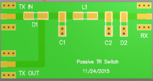
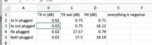
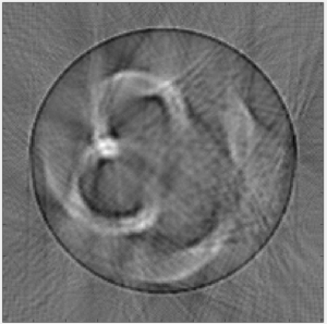
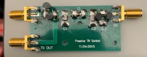
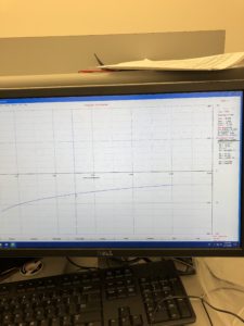
After soldering our T/R switch last week, we needed to verify that it is functioning properly. We did this by measuring the return loss at different ports. We injected a low amplitude, 5 MHz, voltage signal into our switch via the AIM radio, which then also read the signal that was reflected back to it. If all of the signal is reflected, we would get a return loss of 0. When we injected the signal into the Transmit port, we saw a very small return, which indicates that no signal was transmitted. This was expected because a low amplitude voltage should not be enough to turn on the diodes and transmit the signal. When we injected the signal into the Probe port (as if we were reading a signal from the US probe), however, we saw a significant return loss, which means that some of our signal was actually being transmitted to the receiver. These return loss measurements are illustrated in figures 1-5 below.

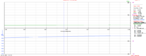
Figure 1. Return loss: antenna connected to TX out, nothing on TX in, 50 ohms on Rx OUT OF BOX

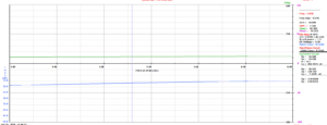
Figure 2. Return loss: antenna connected to Tx out, 50 ohms on Tx in and 50 ohms on Rx OUT OF BOX

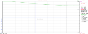
Figure 3. Return loss: antenna connected to Tx in, 50 ohms on Tx and Rx, OUT OF BOX

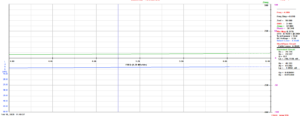
Figure 4. Return loss: antenna connected to Tx out, 50 ohms on Tx in and 50 ohms on Rx IN THE BOX

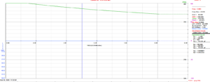
Figure 5. Return loss: antenna connected to Tx in, 50 ohms on Tx and Rx, IN THE BOX

Characterizing the signals for different inputs/outputs of our T/R switch

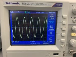
Once we were able to verify that our return loss values matched or expectations, we were also able to characterize our signal with different input/output connections. Using the same AIM radio as a low amplitude, 5 MHz voltage generator, we were able to inject a signal into our T/R switch, and then read the output on an oscilloscope. When we injected the signal into the Transmit port, and measured the signal at the Probe port (with the Receive port loaded with 50 Ohms) we saw a negligible signal, with a peak-to-peak amplitude of 10 mV. This was expected because the low amplitude voltage should not be enough to turn on the diodes and transmit the signal. When we injected the signal into the Probe port, and measured the signal at the Receive port (with the Transmit port loaded with 50 Ohms), we got a signal with a 230 mV peak-to-peak amplitude, which indicates that we are able to measure the signal that would come in from the US probe. The signals received on the oscilloscope are captured in figures 6 and 7 below. 

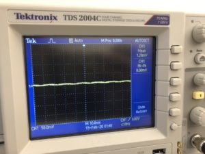
Figure 6. Oscilloscope at Tx out, antenna at Tx in, 50 at Rx, p2p amp =10 mV antenna at Tx out, oscilloscope at Tx in, 50 at Rx, p2p amp = 6 mV

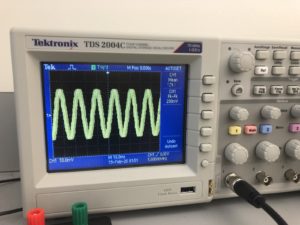
Figure 7. Oscilloscope signal at Rx, antenna at Tx out, 50 at Tx in, p2p amp =230 mV 0 attenuation when device is plugged in.

Creating a 5 MHz function Generator on Ubuntu

Since our AIM radio is limited to only producing low amplitude signals, we needed to create a function generator to transmit a larger signal to the US probe. We were able to create a simple 5 MHz signal using GNU Radio Companion supported by Ubuntu, that we sent through the USRP1 Software Defined Radio and measured with an oscilloscope. The code that was used and the images that were collected can be seen in figures 8-12 below.

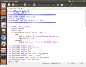
Figure 8

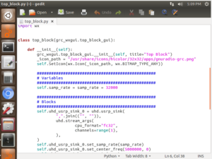
Figure 9

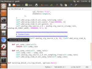
Figure 10

Figures 8-10. The top block Python code generated when the function generator was compiled. 

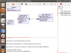
Figure 11

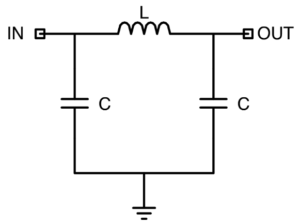
Figure 11. The block diagram of 5MHz function generator with a 500 mV amplitude. 

Questions to answer this week:

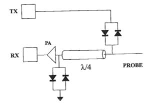
• Question: Under what conditions do each pair of crossed diodes turn on? 
  • Both pairs of diodes turn on under large voltage pulses from the transmitter. Neither pair of diodes is turned on in between the large voltage pulses.

Morgan Kinney, Tanner Hoppman, Jude Franklin

This week while finishing our data acquisition for the IR CT scanner we were able to begin working on our next project, the ultrasound machine. Our first step was creating the phantom to be imaged once we build our ultrasound probe. This was done by combining water with agar and graphite, heating it up in a microwave, and then cooling it and inserting a 3-D printed shape part-way through the cooling process. Next, we built our transmit/receive switch using the board shown in Fig. 1 to match the circuit diagram in Fig. 2 with ceramic chip capacitors, a surface mount inductor, SMA connectors, and four Schottky diodes. The last thing we did was enclose our switch in a metal enclosure for storage so that our next step will be to test it to make sure our soldering has been done properly.

Figure 1. Transmit/Receive switch board used to build T/R switch.

Figure 2. Transmit/Receive switch diagram. The quarter-wave line is modeled through a pi network of two identical capacitors and an inductor.

Question: Under what conditions do each pair of crossed diodes turn on? 

Answer: In Fig. 2, the diodes between TX and the probe turn on when the TX amplifier produces large voltages during transmit to induce a loss of power, and the other diodes turn on when the transducer acts as a source producing small voltage signals during receive.

Week 7

Javier and Nicholas J. Holden

This week was spent on trying to make sure that the TR switch was constructed and functioning properly. Figure 1 shows the soldered circuit. Upon testing the circuit for the first time, we discovered that the inductor was not properly soldered onto the board. This in turn created a break in circuit at the inductor. This was incredibly frustrating because they were difficult to replace due to being delicate. After solving this problem, we then tested that the circuit was continuous. Once this was confirmed we resumed testing for return loss. We encountered a problem when we first did the testing, but we discovered that the error wasn’t from the TR switch but rather the antenna analyzer. This was discovered by testing a working TR switch and observing a very low return loss for Tx-Out with a 50 Ohm load on the Rx port. Figure 2 displays the outer shell of the circuit that was attached with the ports labelled. Upon switching out the analyzer, the return loss was then collected for a variety of situations. This includes a -9.14 dB return signal with the analyzer connected to Tx-Out and a 50 Ohm load on the Rx port. The reverse of this situation was also tested and returned -9.27 dB. This was good as it should be symmetric. When the 50 Ohm load is removed, the return loss in both situations are 0.64 and 0.62 dB. Finally the Tx-In port was tested and had a return loss of .02 dB which is what we expected to occur. Next week, we will get started on running the GNURadio and SDR in order to create a pulse signal as well as familiarizing ourselves with the GNURadio.    

Figure 1

Figure 2

Question: How would you express this mathematically?

Answer: You would express this as an infinite amount of impedance preventing the flow of current. This makes the circuit appear as an open circuit.

Week 7 Blog Post: Ultrasound Scanner

Hunter Spivey and Aayush Gupta

This week we continued working on our T/R switch, and began by calculating our element values necessary for the capacitors and inductor on the T/R switch. After calculating these values, we began soldering the elements on, which was tedious work that took us most of the time we had available. We finished soldering on our elements, but unfortunately had soldered the inductor on upside down, and had to remove and resolder it. Finally we tested our T/R switch using the continuity function of the multimeter, and began setting up our antenna analyzer to test it further. We were able to successfully start and calibrate the antenna analyzer before we ran out of time.

Next we plan on finishing our antenna analyzer tests and moving on the the GNU radio.

T/R switch:

Question: What is the role of the quarter-wave line?

Answer: It changes impedance to allow the path to the RX line to be either a short or open circuit

Question: What values do you get for L and C?

Answer: We get 1.59 microHenris and 636 picoFarads

Myron Mageswaran, Alex Boyd, and Maggie Ford

This week we worked on:

• Testing the T/R Switch we made last week
• Getting familiar with the GNURadio Software

In order to test the return loss at each port (TX input, TX output, and RX), we used the antenna analyzer to inject a 5 MHz signal into each port of the transducer. Before we could do this, however, we had to calibrate the antenna analyzer using a short circuit load, an open circuit load, and a load with an impedance of 50 Ohms. Once the antenna analyzer was calibrated, we connected the oscilloscope to the TX input, TX output, and RX ports and measured the return loss at each port with the antenna analyzer when the other ports had an open connection and when the other ports had a load with an impedance of 50 Ohms. The data we collected suggests that the return loss is nearly zero except when a 5 MHz signal was injected into the TX output port and the resistive load was connected to the RX port, as well as when a 5 MHz port was injected into the RX port and the resistive load was connected to the TX output port. The test data we collected is depicted below.

We spent the remainder of the class period on Thursday setting up the virtual machine with the GNURadio software and familiarizing ourselves with how to use the software. Depicted below is a picture of the software defined radio that we are interfacing with using the Linux virtual machine.

This week, we built our T/R switch and measured power return loss. After calibrating, we measured the power return loss at each port. We got a higher power return loss than expected, so we realized that we accidentally used 6.8 pF capacitors instead of 680 pF capacitors. Then, we used 680 pF through-hole capacitors. Dr. Grissom warned us that he did not know how these capacitors would react to radio frequency, so we replaced these capacitors with the surface mounted ones we were given. Below are the power return losses we observed from each port with the different capacitors.

Through-hole capacitor

Transmit out port

Receive open: 1.32 dB

Receive 50 ohms: 23.05 dB

Receive port

Transmit open: 1.36 ohms

Transmit 50 ohms: 9.46 dB

Surface mounted capacitor

Transmit in port:

Transmit out is open: 0 dB

Transmit out 50 ohms: 0 dB

Transmit out port:

Receive open: 0.77 dB

Receive 50 ohms: 23.57 dB.

Receive port:

Transmit out open. 0.77 dB

Transmit out 50 ohms. 23.31 dB

Figure 1: T/R switch set to 5 MHz input to transmit out looking at receive port

Figure 2: Oscilloscope of T/R switch set to 5 MHz input to transmit out looking at receive port

Question:

With the components we have, how close do you come to satisfying the two conditions above?

We used a 680 pF capacitor and and a 1.5 uH inductor. The capacitor is slightly larger and the inductor is slightly smaller than the desired values.

Morgan Kinney, Tanner Hoppman, Jude Franklin

This week we were unfortunately unable to meet our goal of finishing the IR CT project. After completing another scan, we were able to improve our reconstruction algorithm to obtain the better image quality seen in Fig. 2, but we knew that something else still had to be off. The image is closer to being able to distinguish the phantom used, but after analyzing our sonogram in Fig. 1 we noticed that it is abnormally slanted. At the very end of the week we found the problem: our stepper motor had 200 steps instead of the correct amount of 201. The result is that the stepper motor is one step short of 360 degrees every rotation and our reconstruction gives the image in Fig. 2. With these issues resolved, we are almost certain that our next scans will give better images. We should be able to complete the scans required and move onto our next project (ultrasound) this week.

Figure 1. Image sinogram

Figure 2. Reconstructed image

Question: What happens if you more coarsely or finely sample the fan beam angles?

Answer: Fan beam angles are currently sampled at 1 degree steps. If we were able to sample them more finely, there would be no difference because the stepper motor is the limiting element for resolution since it steps at 1.8 degrees per step. If the fan beam angles were sampled more coarsely than the 1.8 degrees, they would then become the limiting factor and resolution would be negatively impacted.

Blog Post Week #1: Imaging Instrumentation Ultrasound Lab
Jorie Budzikowski, Stephanie Molitor, and Rachel Welscott

(overheard) Quote of the Week:
“Careful, they will draw blood.”

This week we worked on:

I. Making the phantom
II. Soldering the T/R switch
III. Calibrating the AIM Antenna to 50 Ohms

I. Making the Phantom
This week, we were able to prepare a phantom that will be used later in testing. We combined agar, graphite, and water and microwaved the mixture until it was just barely boiling. This allowed all of the ingredients to mix together homogeneously. We stirred the mixture continuously until it cooled to 40 degrees C in order to prevent premature separation of the mixture. As it cooled the rest of the way, we inserted a 3D printed phantom into the beaker, which will be what we ultimately want to image. The graphite and agar surrounding the phantom simply allow the light to be reflected so we receive a realistic signal.

II. Soldering the T/R Switch
The T/R switch consisted of a PCB along with components including two capacitors, two sets of two diodes, and an inductor. Each component was soldered onto the PCB according to the figure below.

Figure 1. Circuit diagram of T/R switch.

Figure 2. Soldered PCB for T/R switch, based off of the above circuit diagram.

The component values for the inductor and capacitor were derived using the desired frequency and impedance values according to the L and C equations below. Using a frequency of 5 MHz, we were able to determine that the ideal capacitance value was 1.6 microHenrys and the ideal inductance value was 636.6 picoFarads.

Equations 1-2. Derivations for inductor (L) and capacitor (C) values used in the T/R switch using a frequency of 5 MHz.

Once it was soldered, the PCB was housed in a steel box (Figure 3) to protect us against the high voltages that will be produced during transmission.

Figure 3. Steel housing that encases the T/R switch during data collection.
III. Calibrating the AIM Antenna to 50 Ohms

The purpose of the AIM Antenna is to send a signal to the transducer and receive the reflected signal back. This measures the return loss, which is the amount of power that is reflected back from the switch at each of the ports of the constructed T/R switch. The AIM Antenna was calibrated using the AIM_916 software on the PC. Following the standard calibration procedure within the program, the antenna was calibrated first using a short circuit, then an open circuit, and finally 50 Ohms to match the impedance of the cables. This calibration was saved and will be used for data collection in the coming weeks.

Questions we aimed to answer this week

1.  What values do you get for L and C?
   1. L=1.6 microHenrys
   2. C= 6.3662e-10 Farads
2. How close can you get to these values with the components we have (without, e.g. using multiple components in each position)?
   1. The actual values we used were limited by those available in the inductor and capacitor kits. We ended up using values of L=1.5 microHenrys and C=680 picoFarads.

Alex Boyd, Myron Mageswaran, Maggie Ford

This week the group began prep work for the Ultrasound scanner.  This started by creating a graphite coating on a 3D printed phantom to later be imaged.  The group also soldered elements to a PCB for the T/R switch to be used by the scanner.  Part of the circuit used is displayed below with the switching diodes arrangement shown in the physical PCB picture.  The L and C values for the T/R switch were solved for using these formulas with 5MHz for f0 and 50 Ohms for Z0:   L = Z0/(2πf0), C = 1/(2πf0Z0).  The group also began calibration of the T/R switch for effective measurement of ultrasound waves when the device is complete, but did not complete the calibration steps.

Figure 1. The transmit/receive switch circuit schematic section with inductors and capacitors

Figure 2. The transmit/receive switch PCB with elements soldered and switching diodes shown.

Question: What values do you get for L and C?

The resulting values were L = 1.59*10^-6 H and C = 636.7 pF which were then rounded to the nearest physical elements available.

This week, we finally obtained a good reconstructed image from our scanner. The trick was adding the function fliplr! Below is our Matlab code and our reconstructed image.

Matlab code

% recon data from an ir ct scanner

%%%%%%%%%%%%%%%%%%%%%%%%%%%

% load the projection data

%%%%%%%%%%%%%%%%%%%%%%%%%%%

% full phantom data – acquired over 360 degrees of stepper motor

load ‘dataTEST_full.txt’; % data file you generate – needs to contain diodeVoltage, servoAngle, and stepAngle

diodeVoltage = dataTEST;

servoAngle = 40:1:128;

stepAngle = 0:1.8:269*1.8;

% %[row col] = size(data);

% outputflipped = zeros(270,89);

% % output = reshape(diodeVoltage, [271 89]);

% outputflipped(2:2:end,:) = fliplr(diodeVoltage(2:2:end,:));

% outputflipped(1:2:end,:) = diodeVoltage(1:2:end,:);

% %odd number rows

% %for ii = 1:2:col/2

%     %output(ii, 🙂 = diodeVoltage(ii, 1:col/2);

% %end

% 

% %even number rows

% for ii = 2:2:col/2

%     output(ii, 🙂 = fliplr(diodeVoltage(ii-1, 1+col/2:col));

% end

%%%%%%%%%%%%%%%%%%%%%%%%%%%

% recon parameters

%%%%%%%%%%%%%%%%%%%%%%%%%%%

N = 128; % matrix size

FOV = 12; % cm, FOV of image matrix

Dcm = 9; % cm, distance from fan beam vertex to center of stepper motor shaft

D = Dcm*N/FOV; % vertex->center distance in pixels

fanCenterAngle = 90; % fan center angle 

fanAngleWidth = 89; % total width we need in degrees for the fan beam to cover the object

%%%%%%%%%%%%%%%%%%%%%%%%%%%

% subtract off the center fan angle from the servo angles, to center them

%%%%%%%%%%%%%%%%%%%%%%%%%%%

servoAngle = servoAngle – fanCenterAngle;

%%%%%%%%%%%%%%%%%%%%%%%%%%%

% reshape data into a fan beam sinogram matrix. We assume that servo angle

% is minor dim in diodeVoltage vector

%%%%%%%%%%%%%%%%%%%%%%%%%%%

nServoAngles = length(unique(servoAngle));

nStepAngles = length(unique(stepAngle));

fanBeamData = diodeVoltage;

%fanBeamData = reshape(diodeVoltage,[nServoAngles,nStepAngles]);

%potVoltage = reshape(potVoltage,[nServoAngles,nStepAngles]);

%%%%%%%%%%%%%%%%%%%%%%%%%%%

% interpolate along the fan beam dimension to center the data

%%%%%%%%%%%%%%%%%%%%%%%%%%%

% find increment between servo Angles

deltaServoAngle = abs(diff(unique(servoAngle)));deltaServoAngle = deltaServoAngle(1);

% find increment between stepper motor angles

deltaStepAngle = abs(diff(unique(stepAngle)));deltaStepAngle = deltaStepAngle(1);

% get input (I) and output (O) interpolation grids

servoAnglesI = min(servoAngle):deltaServoAngle:max(servoAngle);

stepAngles = min(stepAngle):deltaStepAngle:max(stepAngle);

[stepAnglesI,servoAnglesI] = meshgrid(stepAngles,servoAnglesI);

servoAnglesO = -fanAngleWidth/2:fanAngleWidth/2;

stepAngles = min(stepAngle):deltaStepAngle:360-1.8;

[stepAnglesO,servoAnglesO] = meshgrid(stepAngles,servoAnglesO);

% do the 2D interpolation to the centered grid that we will use for recon

fanBeamDataCent = interp2(stepAnglesI, servoAnglesI, fanBeamData’, stepAnglesO, servoAnglesO, ‘cubic’, 0);

%servoAnglesI’, stepAnglesI’, fanBeamData,servoAnglesO’,stepAnglesO’,’cubic’,255);

%fanBeamDataCent(fanBeamDataCent > 100) = 255;

%sinogram

figure;imagesc(abs(fanBeamDataCent));

title(‘Sinogram’);

xlabel(‘Angle (degrees)’);

ylabel(‘Distance (cm)’);

colorbar 

%%%%%%%%%%%%%%%%%%%%%%%%%%%

% reconstruct the image

%%%%%%%%%%%%%%%%%%%%%%%%%%%

 img = ifanbeam(fliplr(fanBeamDataCent),D,’fancoverage’,’cycle’,’fanrotationincrement’,…

    deltaStepAngle,’fansensorgeometry’,’arc’,’fansensorspacing’,1,…

    ‘filter’,’Ram-Lak’,’frequencyscaling’,1,’interpolation’,’nearest’,…

    ‘outputsize’,N);

figure;imagesc(-img);axis image;colormap gray

title(‘Reconstructed Image’);

We also began to make our ultrasound scanner. We re-made the agar graphite phantom, since our phantom from last week separated into layers, and we soldered photodiodes, capacitors, inductors, and connectors onto our PCB board for the transmit/receive switch. Next, we used a windows software to  measure the power return loss of the switch. We found a 17 dB return loss. The set up of the T/R switch connected to the hardware and a screenshot of the frequency curve is shown below.

Question:

What values do you get for L and C?

L = 1.59  uH

C = 637 pF