Alex Boyd, Maggie Ford, and Myron Mageswaran
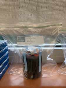
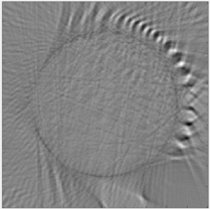
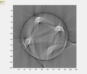
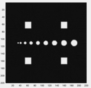
The construction of the actual scanner was completed in previous labs, so the past week was spent mostly collecting data and then polishing the MATLAB code to try to improve the reconstructed image. The first image collected (Image 1) was overall somewhat clear, but for a portion of the collection, the photodiode was unplugged, so the image contains a blurry spot from the incorrect data points. Students then took another complete data set to use for the reconstruction. This new image (Image 2) was very clear, but had a bit of a ring around the object. To correct this, students remeasured, adjusted, and tested the FOV and other parameters and used the best corresponding values.
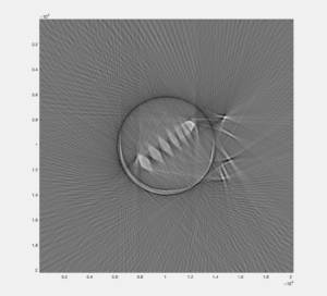
Image 1: The first image students reconstructed using the data set that had the photodiode disconnected for a portion of time evidenced by the region circled on the right side
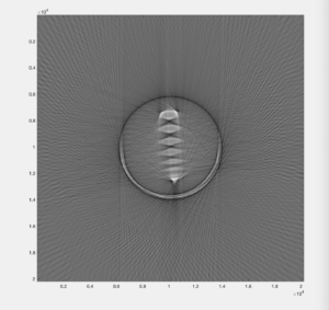
Image 2: The new image students reconstructed using the complete data set
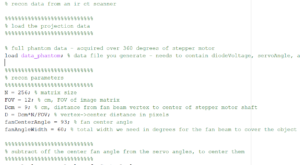
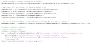
MATLAB CODE: Below is the code that students used for the reconstruction of the images with comments to follow along
%Reconstruction of an Infrared CT Scanner
%%%%%%%%%%%%%%%%%%%%%%%%%%%
% load the projection data
%%%%%%%%%%%%%%%%%%%%%%%%%%%
% full phantom data – acquired over 360 degrees of stepper motor
load phantom2Trial1.mat; % data file you generate – needs to contain diodeVoltage, servoAngle, and stepperAngle
%%%%%%%%%%%%%%%%%%%%%%%%%%%
% recon parameters
%%%%%%%%%%%%%%%%%%%%%%%%%%%
N = 20200; % matrix size
FOV = 17.45; % cm, FOV of image matrix
Dcm = 7.78; % cm, distance from fan beam vertex to center of stepper motor shaft
D = Dcm*N/FOV; % vertex->center distance in pixels
fanCenterAngle = 80; % fan center angle
fanAngleWidth = 100; % total width we need in degrees for the fan beam to cover the object
%%%%%%%%%%%%%%%%%%%%%%%%%%%
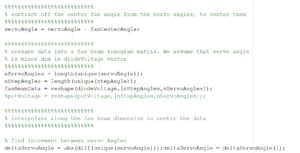
% subtract off the center fan angle from the servo angles, to center them
%%%%%%%%%%%%%%%%%%%%%%%%%%%
servoAngle = servoAngle – fanCenterAngle;
%%%%%%%%%%%%%%%%%%%%%%%%%%%
% reshape data into a fan beam sinogram matrix. We assume that servo angle
% is minor dim in diodeVoltage vector
%%%%%%%%%%%%%%%%%%%%%%%%%%%
nServoAngles = length(unique(servoAngle));
nStepAngles = length(unique(stepperAngle));
fanBeamData = reshape(diodeVoltage,[nServoAngles,nStepAngles]);
% potVoltage = reshape(potVoltage,[nServoAngles,nStepAngles]);
%%%%%%%%%%%%%%%%%%%%%%%%%%%
% interpolate along the fan beam dimension to center the data
%%%%%%%%%%%%%%%%%%%%%%%%%%%
% find increment between servo Angles
deltaServoAngle = abs(diff(unique(servoAngle)));
deltaServoAngle = deltaServoAngle(1);
% find increment between stepper motor angles
deltaStepAngle = abs(diff(unique(stepperAngle)));
deltaStepAngle = deltaStepAngle(1);
% get input (I) and output (O) interpolation grids
servoAnglesI = min(servoAngle):deltaServoAngle:max(servoAngle);
stepAngles = min(stepperAngle):deltaStepAngle:max(stepperAngle);
[stepAnglesI,servoAnglesI] = meshgrid(stepAngles,servoAnglesI);
servoAnglesO = -fanAngleWidth/2:fanAngleWidth/2;
[stepAnglesO,servoAnglesO] = meshgrid(stepAngles,servoAnglesO);
% do the 2D interpolation to the centered grid that we will use for recon
fanBeamDataCent = interp2(stepAnglesI,servoAnglesI,fanBeamData,stepAnglesO,servoAnglesO,’cubic’,0);
%%%%%%%%%%%%%%%%%%%%%%%%%%%
% reconstruct the image
%%%%%%%%%%%%%%%%%%%%%%%%%%%
img = ifanbeam(fliplr(fanBeamDataCent),D,’fancoverage’,’cycle’,’fanrotationincrement’,…
deltaStepAngle,’fansensorgeometry’,’arc’,’fansensorspacing’,1,…
‘filter’,’Ram-Lak’,’frequencyscaling’,1,’interpolation’,’nearest’,…
‘outputsize’,N);
figure;imagesc(-img);axis image;colormap gray
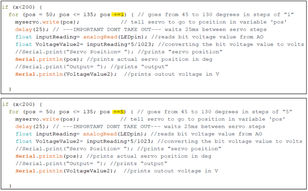
Question 1:
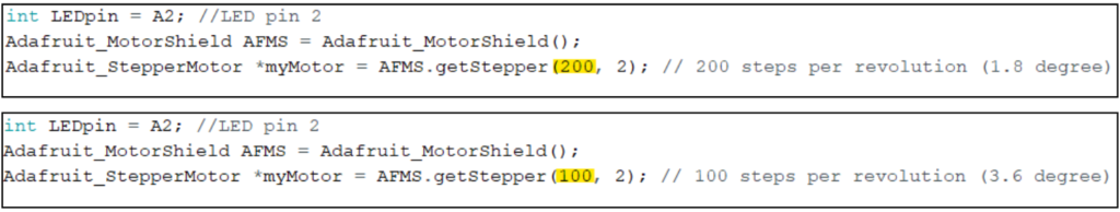
What happens if you more coarsely or finely sample the stepper motor positions? The finer the stepper motor position, the higher resolution of the image because there are more data points.

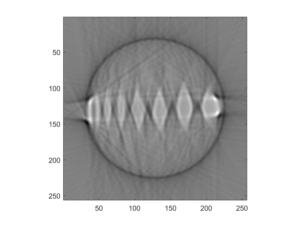
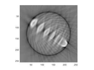
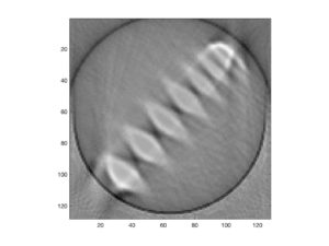
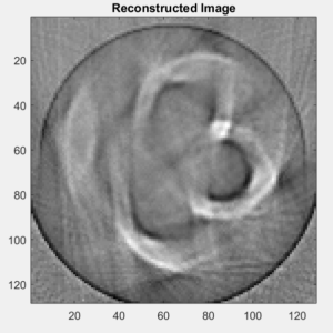
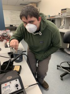 Figure 1 – Javier stirring the graphite/auger mixture