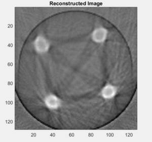
This week, we finally obtained a good reconstructed image from our scanner. The trick was adding the function fliplr! Below is our Matlab code and our reconstructed image.
Matlab code
% recon data from an ir ct scanner
%%%%%%%%%%%%%%%%%%%%%%%%%%%
% load the projection data
%%%%%%%%%%%%%%%%%%%%%%%%%%%
% full phantom data – acquired over 360 degrees of stepper motor
load ‘dataTEST_full.txt’; % data file you generate – needs to contain diodeVoltage, servoAngle, and stepAngle
diodeVoltage = dataTEST;
servoAngle = 40:1:128;
stepAngle = 0:1.8:269*1.8;
% %[row col] = size(data);
% outputflipped = zeros(270,89);
% % output = reshape(diodeVoltage, [271 89]);
% outputflipped(2:2:end,:) = fliplr(diodeVoltage(2:2:end,:));
% outputflipped(1:2:end,:) = diodeVoltage(1:2:end,:);
% %odd number rows
% %for ii = 1:2:col/2
% %output(ii, 🙂 = diodeVoltage(ii, 1:col/2);
% %end
%
% %even number rows
% for ii = 2:2:col/2
% output(ii, 🙂 = fliplr(diodeVoltage(ii-1, 1+col/2:col));
% end
%%%%%%%%%%%%%%%%%%%%%%%%%%%
% recon parameters
%%%%%%%%%%%%%%%%%%%%%%%%%%%
N = 128; % matrix size
FOV = 12; % cm, FOV of image matrix
Dcm = 9; % cm, distance from fan beam vertex to center of stepper motor shaft
D = Dcm*N/FOV; % vertex->center distance in pixels
fanCenterAngle = 90; % fan center angle
fanAngleWidth = 89; % total width we need in degrees for the fan beam to cover the object
%%%%%%%%%%%%%%%%%%%%%%%%%%%
% subtract off the center fan angle from the servo angles, to center them
%%%%%%%%%%%%%%%%%%%%%%%%%%%
servoAngle = servoAngle – fanCenterAngle;
%%%%%%%%%%%%%%%%%%%%%%%%%%%
% reshape data into a fan beam sinogram matrix. We assume that servo angle
% is minor dim in diodeVoltage vector
%%%%%%%%%%%%%%%%%%%%%%%%%%%
nServoAngles = length(unique(servoAngle));
nStepAngles = length(unique(stepAngle));
fanBeamData = diodeVoltage;
%fanBeamData = reshape(diodeVoltage,[nServoAngles,nStepAngles]);
%potVoltage = reshape(potVoltage,[nServoAngles,nStepAngles]);
%%%%%%%%%%%%%%%%%%%%%%%%%%%
% interpolate along the fan beam dimension to center the data
%%%%%%%%%%%%%%%%%%%%%%%%%%%
% find increment between servo Angles
deltaServoAngle = abs(diff(unique(servoAngle)));deltaServoAngle = deltaServoAngle(1);
% find increment between stepper motor angles
deltaStepAngle = abs(diff(unique(stepAngle)));deltaStepAngle = deltaStepAngle(1);
% get input (I) and output (O) interpolation grids
servoAnglesI = min(servoAngle):deltaServoAngle:max(servoAngle);
stepAngles = min(stepAngle):deltaStepAngle:max(stepAngle);
[stepAnglesI,servoAnglesI] = meshgrid(stepAngles,servoAnglesI);
servoAnglesO = -fanAngleWidth/2:fanAngleWidth/2;
stepAngles = min(stepAngle):deltaStepAngle:360-1.8;
[stepAnglesO,servoAnglesO] = meshgrid(stepAngles,servoAnglesO);
% do the 2D interpolation to the centered grid that we will use for recon
fanBeamDataCent = interp2(stepAnglesI, servoAnglesI, fanBeamData’, stepAnglesO, servoAnglesO, ‘cubic’, 0);
%servoAnglesI’, stepAnglesI’, fanBeamData,servoAnglesO’,stepAnglesO’,’cubic’,255);
%fanBeamDataCent(fanBeamDataCent > 100) = 255;
%sinogram
figure;imagesc(abs(fanBeamDataCent));
title(‘Sinogram’);
xlabel(‘Angle (degrees)’);
ylabel(‘Distance (cm)’);
colorbar
%%%%%%%%%%%%%%%%%%%%%%%%%%%
% reconstruct the image
%%%%%%%%%%%%%%%%%%%%%%%%%%%
img = ifanbeam(fliplr(fanBeamDataCent),D,’fancoverage’,’cycle’,’fanrotationincrement’,…
deltaStepAngle,’fansensorgeometry’,’arc’,’fansensorspacing’,1,…
‘filter’,’Ram-Lak’,’frequencyscaling’,1,’interpolation’,’nearest’,…
‘outputsize’,N);
figure;imagesc(-img);axis image;colormap gray
title(‘Reconstructed Image’);

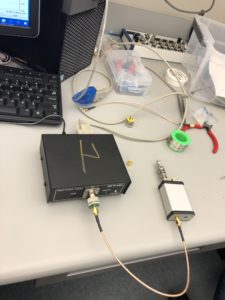
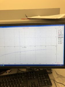
We also began to make our ultrasound scanner. We re-made the agar graphite phantom, since our phantom from last week separated into layers, and we soldered photodiodes, capacitors, inductors, and connectors onto our PCB board for the transmit/receive switch. Next, we used a windows software to measure the power return loss of the switch. We found a 17 dB return loss. The set up of the T/R switch connected to the hardware and a screenshot of the frequency curve is shown below.


Question:
What values do you get for L and C?
L = 1.59 uH
C = 637 pF
