Blog Post Week #2: Imaging Instrumentation Ultrasound Lab

Jorie Budzikowski, Stephanie Molitor, and Rachel Welscott

(overheard) QUOTE OF THE WEEK: 

“Everything is a learning experience”

This week we worked on: 

1. Measuring the return loss of our T/R switch
2. Characterizing the signals for different inputs/outputs of our T/R switch
3. Making a 5 MHz function generator on Ubuntu

Measuring the return loss of our T/R switch

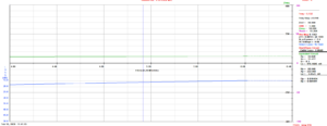
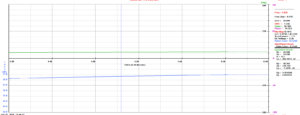
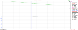
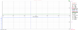
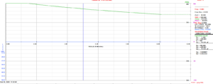
After soldering our T/R switch last week, we needed to verify that it is functioning properly. We did this by measuring the return loss at different ports. We injected a low amplitude, 5 MHz, voltage signal into our switch via the AIM radio, which then also read the signal that was reflected back to it. If all of the signal is reflected, we would get a return loss of 0. When we injected the signal into the Transmit port, we saw a very small return, which indicates that no signal was transmitted. This was expected because a low amplitude voltage should not be enough to turn on the diodes and transmit the signal. When we injected the signal into the Probe port (as if we were reading a signal from the US probe), however, we saw a significant return loss, which means that some of our signal was actually being transmitted to the receiver. These return loss measurements are illustrated in figures 1-5 below.

Figure 1. Return loss: antenna connected to TX out, nothing on TX in, 50 ohms on Rx OUT OF BOX

Figure 2. Return loss: antenna connected to Tx out, 50 ohms on Tx in and 50 ohms on Rx OUT OF BOX

Figure 3. Return loss: antenna connected to Tx in, 50 ohms on Tx and Rx, OUT OF BOX

Figure 4. Return loss: antenna connected to Tx out, 50 ohms on Tx in and 50 ohms on Rx IN THE BOX

Figure 5. Return loss: antenna connected to Tx in, 50 ohms on Tx and Rx, IN THE BOX

Characterizing the signals for different inputs/outputs of our T/R switch

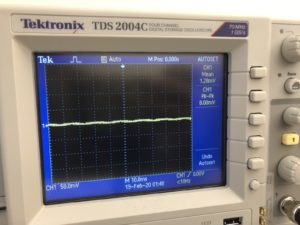
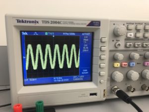
Once we were able to verify that our return loss values matched or expectations, we were also able to characterize our signal with different input/output connections. Using the same AIM radio as a low amplitude, 5 MHz voltage generator, we were able to inject a signal into our T/R switch, and then read the output on an oscilloscope. When we injected the signal into the Transmit port, and measured the signal at the Probe port (with the Receive port loaded with 50 Ohms) we saw a negligible signal, with a peak-to-peak amplitude of 10 mV. This was expected because the low amplitude voltage should not be enough to turn on the diodes and transmit the signal. When we injected the signal into the Probe port, and measured the signal at the Receive port (with the Transmit port loaded with 50 Ohms), we got a signal with a 230 mV peak-to-peak amplitude, which indicates that we are able to measure the signal that would come in from the US probe. The signals received on the oscilloscope are captured in figures 6 and 7 below. 

Figure 6. Oscilloscope at Tx out, antenna at Tx in, 50 at Rx, p2p amp =10 mV antenna at Tx out, oscilloscope at Tx in, 50 at Rx, p2p amp = 6 mV

Figure 7. Oscilloscope signal at Rx, antenna at Tx out, 50 at Tx in, p2p amp =230 mV 0 attenuation when device is plugged in.

Creating a 5 MHz function Generator on Ubuntu

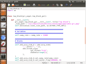
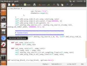
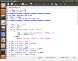
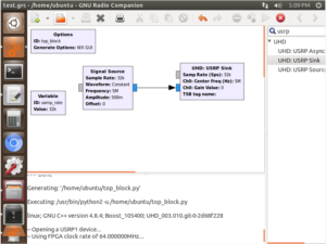
Since our AIM radio is limited to only producing low amplitude signals, we needed to create a function generator to transmit a larger signal to the US probe. We were able to create a simple 5 MHz signal using GNU Radio Companion supported by Ubuntu, that we sent through the USRP1 Software Defined Radio and measured with an oscilloscope. The code that was used and the images that were collected can be seen in figures 8-12 below.

Figure 8

Figure 9

Figure 10

Figures 8-10. The top block Python code generated when the function generator was compiled. 

Figure 11

Figure 11. The block diagram of 5MHz function generator with a 500 mV amplitude. 

Questions to answer this week:

• Question: Under what conditions do each pair of crossed diodes turn on? 
  • Both pairs of diodes turn on under large voltage pulses from the transmitter. Neither pair of diodes is turned on in between the large voltage pulses.

Blog Post Week #4: Imaging Instrumentation Infrared CT Lab                                   Jorie Budzikowski, Stephanie Molitor, and Rachel Welscott

(overheard) QUOTE OF THE WEEK:                                                                         “Have you ever seen a CT scanner without a hood on it?”                                                “…Yes we had to watch that for THIS class”

Because of our progress last week with optimizing the servo and stepper motor’s rotation, we were able to make progress this week on:

1. Matlab code to collect the voltage and position vectors needed for image reconstruction
2. Image reconstruction in Matlab
   
   

1. Collecting the voltage and position vectors in Matlab

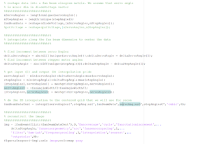
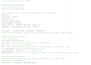
Our arduino code that controls the stepper motor and servo rotation also prints their positions and the voltage values collected at each position. Moving into Matlab, our code reads off of the serial monitor from the arduino and produces a single vector with values that alternate the servo angle and the diode voltage at that position. We were then able to extract the position and the voltage values from that vector by taking the values for either the even or odd indices. Image one shows the actual code that is used to collect the vectors. These are the two vectors (theta and voltage) that are necessary to reconstruct the image. Additionally, we manually constructed a vector of our relative stepper motor angles by using the step size of 1.8 degrees that we previously calculated. 

It takes about 10 minutes to collect a complete dataset, as the servo motor scans the phantom 200 times, once for each step of the stepper motor to complete a 360 degree turn. This results in a total vector length of 17,200 data points for each of the three (servo angle, stepper angle, and voltage) vectors. We completed this data acquisition in class. 

Video 1: Stepper and servo motor rotating during data collection

IMG_2152 (1)

2. Image reconstruction in Matlab

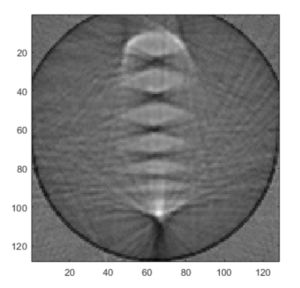
Using the template for image reconstruction in Matlab, we were able to input our data collected for voltage, stepper angle, and servo angle along with some physical constraints of our system and desired output image. We had to convert our single detector voltages into fan beam data in order to reconstruct the sinograms from our voltages. From here, we simply used the radon function in Matlab to convert our sinograms to an image. The reconstructed image still has some slight parameter changes necessary to optimize the image, however the output image looks like our phantom! We will continue to alter the fan center angle and width to increase resolution, and  test our system on other phantoms in the upcoming week.

Image 1: Code for the Matlab reconstruction (using template)

Image 2: The reconstructed image of the phantom

Questions

• Image Errors
  • Question: Do all the features in your phantom images have the correct size? If not, why? Are their sizes accurately represented in all dimensions?
    • No, not all the features in the phantom image have the correct size. Our phantom image is much more rounded than the rectangular extrusions of our phantom. The overall size and spacing of our phantom image reflect our actual phantom, but the fine details (especially corners) are distorted.
• Artifacts and Resolution
  • Question: What happens if you more coarsely or finely sample the fan beam angle and/or stepper motor positions?
    • Currently, the stepper motor has a step angle of 1.8 degrees and our servo has a step angle of 1 degree for each measurement taken. This makes our stepper motor the limiting factor with spatial resolution. We think that by more finely sampling the servo, we would see no change in image resolution because the servo is not the current limiting factor. However, by  more finely sampling the stepper motor, we would be able to increase the spatial resolution of our image and perhaps better image the finer details of our phantom.

Jorie Budzikowski, Stephanie Molitor, and Rachel Welscott

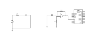
This week we designed a two circuits, one to power the Infrared LED and the second to amplify the signal received by the photodiode. We also began to test the signal from the IR to the photodiode and physically implemented both of these circuits onto the servo itself. Our designed circuit consists of two parts, the first of which is an infrared LED circuit. The IR LED is powered by a 5 V supplied by the Arduino Uno. A resistor separates the LED from the power supply to ensure that too much voltage is not applied across the LED damaging it. The second half of the circuit is a current-to-voltage converter. The photodiode receives light emitted from the IR LED, which results in a current output from the photodiode. This current is directed into the positive terminal of the op amp. The noninverting op amp has a feedback resistor that amplifies this input and results in an output voltage proportional to the current supplied by the photodiode. This essentially converts the IR from the LED to voltage that can be recorded by the Arduino.

The circuit design on our breadboard and Arduino is as shown in the schematic below:

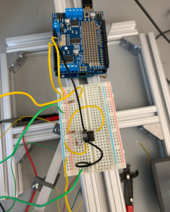
The circuit diagram implemented onto the breadboard and the Arduino:

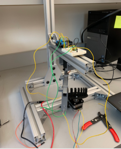
Finally, the entire servo, circuit, Arduino, and phantom together:

Next week, we will continue to finalize the circuit design and program the Arduino to communicate with the servo.