Blog Post Week #3: Imaging Instrumentation Ultrasound Lab
Jorie Budzikowski, Stephanie Molitor, and Rachel Welscott

This week we worked on:
I. Making a pulse-echo sequence
II. Programming the Servo to sweep through a range of angles for B-mode imaging
III. Finalized our setup prior to data acquisition

I. Making a pulse-echo sequence
Once we got a basic sinusoidal function generator functioning through the GNU Radio software (Figure 1), we were able to alter the conditions of the signal source to create pulses that are 1 microsecond in duration. We are able to do so by introducing a delay, a multiplier, and an additional function to our square wave source. The pulse is sent to the radio, will be amplified, and then transmitted through the ultrasound probe. We also added a radio source and GUI sink component in order to read what signal is reflected back from the ultrasound transducer. The block diagram for our pulse-echo sequence is shown in Figure 2.

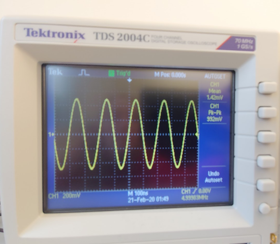Figure 1. Simple 5 MHz sinusoidal signal from our function generator using the USRP radio.

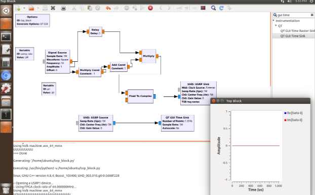Figure 2. Block diagram for our pulse-echo sequence.

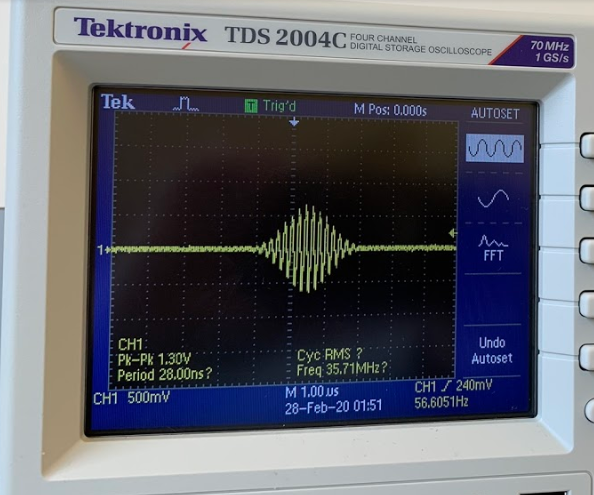Figure 3. Oscilloscope readout of our 1 us pulse signal from the URSP radio.

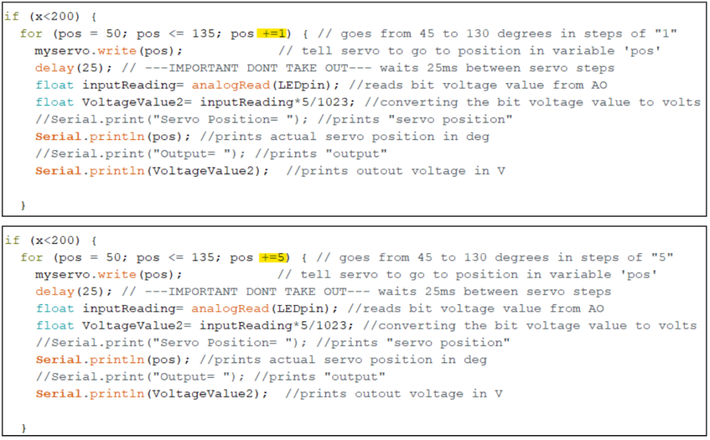
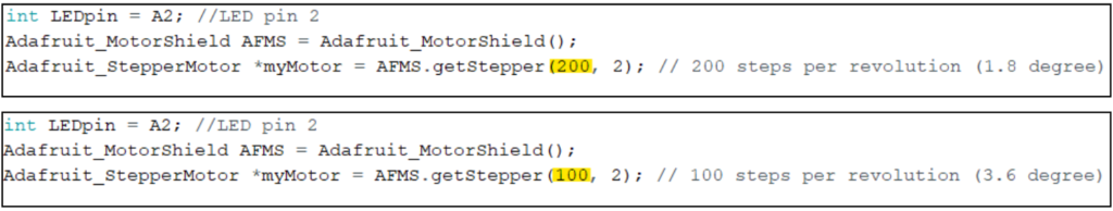
II. Programming the Servo to sweep through a range of angles for B-mode imaging
The arduino was programmed to move to the angle plugged into the serial monitor. The servo object was first created and the serial monitor was initialized. The position variable (pos) was initialized and set equal to the read in value that was entered into the serial monitor. Next we used an if statement to ensure that the value that was inputted into the serial monitor is attainable by the servo motor. Finally, the inputted position was written to the servo motor so that ultrasound probe was pointed at the intended angle. See the attached video of our servo moving the ultrasound transducer.

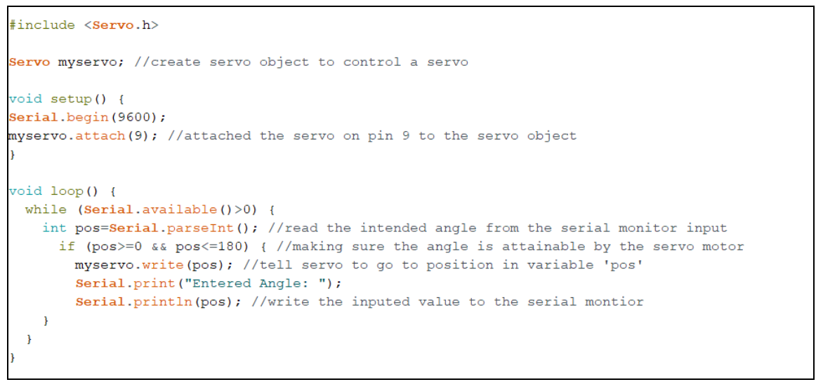Figure 4. Arduino code to control the servo arm and have it move to a desired angle.

III. Final Equipment Setup Prior to Data Acquisition
Now that we have programmed our URSP radio to transmit and receive signals, and programmed our servo arm to move the transducer, we are ready to start collecting some ultrasound data!

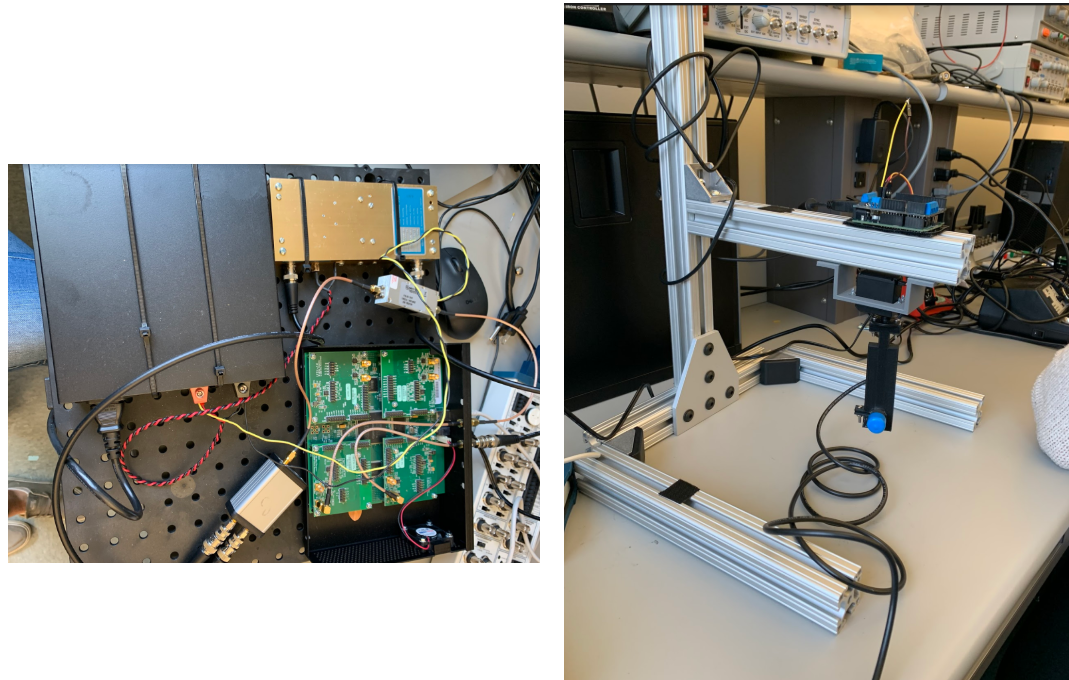Figure 5-6. The electronics of the ultrasound probe system and the physical probe-stand tabletop model.

Questions to answer this week:

• Question: How can you do this using a single square wave signal source, a delay, and a signal multiply block?
  • You can send the single pulse as an input into two different operator functions. One of the functions should not do anything to the waveform while the other function adds a delay and a multiplication constant. These 2 new wave forms are then multiplied together to result in a square waveform with a very short pulse width.
• Question: The simplest solution using the above three elements has an upper limit on the pulse repetition time, because of the very large delays required. How can you modify it so that you can use only a 1 us delay?
  • The simplest solution only involves the signal source, a delay, and a multiplier. We originally planned to use a large delay with this setup; however, due to the upper limit we found that we had to modify our design. We instead changed the used a short delay in combination with an addition operation to get a 1 us delay.

Blog Post Week #1: Imaging Instrumentation Ultrasound Lab
Jorie Budzikowski, Stephanie Molitor, and Rachel Welscott

(overheard) Quote of the Week:
“Careful, they will draw blood.”

This week we worked on:

I. Making the phantom
II. Soldering the T/R switch
III. Calibrating the AIM Antenna to 50 Ohms

I. Making the Phantom
This week, we were able to prepare a phantom that will be used later in testing. We combined agar, graphite, and water and microwaved the mixture until it was just barely boiling. This allowed all of the ingredients to mix together homogeneously. We stirred the mixture continuously until it cooled to 40 degrees C in order to prevent premature separation of the mixture. As it cooled the rest of the way, we inserted a 3D printed phantom into the beaker, which will be what we ultimately want to image. The graphite and agar surrounding the phantom simply allow the light to be reflected so we receive a realistic signal.

II. Soldering the T/R Switch
The T/R switch consisted of a PCB along with components including two capacitors, two sets of two diodes, and an inductor. Each component was soldered onto the PCB according to the figure below.

Figure 1. Circuit diagram of T/R switch.

Figure 2. Soldered PCB for T/R switch, based off of the above circuit diagram.

The component values for the inductor and capacitor were derived using the desired frequency and impedance values according to the L and C equations below. Using a frequency of 5 MHz, we were able to determine that the ideal capacitance value was 1.6 microHenrys and the ideal inductance value was 636.6 picoFarads.

Equations 1-2. Derivations for inductor (L) and capacitor (C) values used in the T/R switch using a frequency of 5 MHz.

Once it was soldered, the PCB was housed in a steel box (Figure 3) to protect us against the high voltages that will be produced during transmission.

Figure 3. Steel housing that encases the T/R switch during data collection.
III. Calibrating the AIM Antenna to 50 Ohms

The purpose of the AIM Antenna is to send a signal to the transducer and receive the reflected signal back. This measures the return loss, which is the amount of power that is reflected back from the switch at each of the ports of the constructed T/R switch. The AIM Antenna was calibrated using the AIM_916 software on the PC. Following the standard calibration procedure within the program, the antenna was calibrated first using a short circuit, then an open circuit, and finally 50 Ohms to match the impedance of the cables. This calibration was saved and will be used for data collection in the coming weeks.

Questions we aimed to answer this week

1.  What values do you get for L and C?
   1. L=1.6 microHenrys
   2. C= 6.3662e-10 Farads
2. How close can you get to these values with the components we have (without, e.g. using multiple components in each position)?
   1. The actual values we used were limited by those available in the inductor and capacitor kits. We ended up using values of L=1.5 microHenrys and C=680 picoFarads.

Jorie Budzikowski, Stephanie Molitor, and Rachel Welscott

This week we were able to work on:

1. Imaging various phantoms
2. Changing image collection parameters including step size, light around the detector, field of view, etc.

1. Imaging Various Phantoms

Last week we were able to complete our servo, stepper motor, and Arduino code. We also were able to complete the image reconstruction of our first phantom. This week we aimed to continue to gather data with different phantoms and altered parameters on the image reconstruction script including the field of view, fan angle width, and distance from the center of the phantom to the servo motor to get a clear image. Some of the relevant image parameters we aimed to investigate were the image resolution, the smallest detectable line pair, image artifacts, and image scale size. The actual code changes for this week are minimal, but the changes to the sinogram and the corresponding phantom image were significant.

We were able to make reconstructions of three different phantoms, shown below. The overall quality of these reconstructions is decent, as we were able to discern the general shapes and spacing. However, some distortions were present, such as blurring of edges that turned square shapes more round. Additionally, we found the second phantom (middle image below) produced the least clear reconstruction. We found that this was due to the outer four pegs blocking the IR light from the inner pegs. Since our CT scanner only took images in one direction at a time, this altered our final reconstructed image.

Image 1: The three different phantoms we were able to produce images of using our Infrared CT scanner system.
2. Changing Image Collection Parameters
We also changed the step size for both the servo and the stepper motor to determine how the step size correlated to image resolution. We changed the servo step size from 1 to 5 degrees, and changed the stepper motor from 1.8 to 3.6 degrees. We were able to change the step size very easily, by only changing one value in our Arduino code, as shown below. We determined that an increased step size for both the servo and of the stepper motor resulted in a decreased image resolution, as illustrated in the following image reconstructions.

Image 2: Increasing the servo step size (left) and increasing the stepper motor step size (right), both had the effect of decreasing image resolution.

Image 3: The Arduino code, showing the parameter changes to alter the step size of the servo from a step size of 1 (top) to a step size of 5 degrees (bottom).

Image 4: The Arduino code, showing the parameter changes to alter the step size of the stepper motor from a step size of 1.8 (top) to a step size of 3.6 degrees (bottom).

The next parameter we changed was the lighting around our detector. We were working by the window, so we found that the generated sinogram showed different colors on the window side and classroom side of the image. This would impact the resolution of our image reconstructions by changing the grayscale coloring of the phantom. By covering our CT scanner with jackets to block the light during the collection, we were able to eliminate this variability in coloring of the image due to the lighting and produce a more consistent ambient environment signal.
Additionally, one of the artifacts that we noticed in our reconstruction was a dark ring around the outside of each phantom (see Image 1). We believe that this was due to a high level of noise at the upper end of our fan angle. This is easily seen by the blue stripe on the far right of our sinograms. By cropping the fan angle in our reconstruction to only capture the bulk of the sinogram, we were able to make this dark ring less apparent.

Image 5: Two sinograms produced from an unlit (left) environment and an environment with ambient light (right). Both sinograms feature a dark blue stripe on the far right, which is what produced the dark ring around our image reconstructions.

The questions that we aimed to answer in this lab are as follows:

1. What is the smallest feature or line pair that you can resolve?
   1. The smallest gap between phantom pegs that we were able to resolve in our image reconstruction was measured to be 0.445 inches.
2. What happens if you more coarsely or finely sample the fan beam angle and/or stepper motor positions?
   1. Last week, we hypothesized that a smaller step size for the servo and stepper motor would produce finer spatial resolution. This week, we were able to test our hypothesis and found that we were correct, as increasing the step size of each resulted in a very poor image reconstruction.

Blog Post Week #3: Imaging Instrumentation Infrared CT Lab
Jorie Budzikowski, Stephanie Molitor, and Rachel Welscott

Quote of the Week:

“Do you know what this delay is for?”
“I don’t know, but it’s probably not important. You can delete it.”
*deletes delay*
…
“OKAY so that delay was VERY important!”

This week, we were able to tackle several parts of the Infrared CT Scanner including the servo rotation, the stepper motor rotation, and the Matlab readout of photodiode voltage from the Arduino.

The Servo and Stepper Rotation:

With the success of the voltage readouts from our circuit, we have since turned our attention to the Servo that controls the rotating arm of the scanner. We have programmed the Servo (via Arduino) to move the rotating arm, and have optimized the speed and delay during rotation. The code that controls the Servo rotation is shown in the image below. We have also programmed the stepper motor to move the phantom with a step size of 1.8 degrees between each full sweep of the servo arm. To complete a full 360 degree image of the phantom, the stepper motor must rotate the phantom 200 times. The combined movements from the Servo and the stepper motor are shown in the video below. We have also altered the Arduino code to display the output voltage and sweeper arm position on the serial monitor for each data point.

Video one: The Servo has been programmed to rotate the sweeper arm around the phantom, and the stepper motor takes (very small) steps between each full sweep.

Image One: The Arduino code that controls both Servo and stepper motor rotation. This code also writes the output voltage and corresponding sweeper arm position to the serial monitor.

The Matlab readout of the photodiode voltage from the Arduino:

Matlab is a crucial element to this CT Infrared Scanner because it is the way that we will ultimately analyze the results from our scan. Our code should read out and store the voltage value at each point for both the sweeper arm and gantry rotation. These readout values will be translated into binary numbers and be displayed as black or white on our image reconstruction. Our preliminary code, shown below, is used to read and store the output voltage for each step of our Servo and stepper motor.

Image Two: The Matlab code that stores the output voltage value for each step.

Questions we set out to answer this week:

1. What is the finest resolution with which you can move the swing arm (servo) and stage (stepper motor)? What does this dictate about the finest spatial resolution of your image?
   1. The smallest step size that we can take with the stepper motor is 1.8 degrees. The smallest step size we can take with the servo is 1 degree. This dictates that the finest spatial resolution of our image is 1.8 degrees since this is the larger of the two component resolution values.
2. The servo has an extra (white) wire on it, that reads out its built-in position potentiometer, which you can use to record the servo’s actual position (rather than just its intended position). Is your image reconstruction improved by using this value instead of the intended value?
   1. The position value of the servo is an arbitrary position value. As long as we know where the designated 0 position is located, it does not really matter whether or not we know the actual position of the servo. Thus, the white wire does not add much information to our system.
3. What parameters of your scanner and scan method influence resolution? Investigate these.
   1. The parameters that influence resolution are the step size of the servo motor and the time the servo motor has to record a section of the “image” in between steps.