Myron Mageswaran, Alex Boyd, and Maggie Ford

This week we worked on:

• Testing the T/R Switch we made last week
• Getting familiar with the GNURadio Software

In order to test the return loss at each port (TX input, TX output, and RX), we used the antenna analyzer to inject a 5 MHz signal into each port of the transducer. Before we could do this, however, we had to calibrate the antenna analyzer using a short circuit load, an open circuit load, and a load with an impedance of 50 Ohms. Once the antenna analyzer was calibrated, we connected the oscilloscope to the TX input, TX output, and RX ports and measured the return loss at each port with the antenna analyzer when the other ports had an open connection and when the other ports had a load with an impedance of 50 Ohms. The data we collected suggests that the return loss is nearly zero except when a 5 MHz signal was injected into the TX output port and the resistive load was connected to the RX port, as well as when a 5 MHz port was injected into the RX port and the resistive load was connected to the TX output port. The test data we collected is depicted below.

We spent the remainder of the class period on Thursday setting up the virtual machine with the GNURadio software and familiarizing ourselves with how to use the software. Depicted below is a picture of the software defined radio that we are interfacing with using the Linux virtual machine.

This week, we built our T/R switch and measured power return loss. After calibrating, we measured the power return loss at each port. We got a higher power return loss than expected, so we realized that we accidentally used 6.8 pF capacitors instead of 680 pF capacitors. Then, we used 680 pF through-hole capacitors. Dr. Grissom warned us that he did not know how these capacitors would react to radio frequency, so we replaced these capacitors with the surface mounted ones we were given. Below are the power return losses we observed from each port with the different capacitors.

Through-hole capacitor

Transmit out port

Receive open: 1.32 dB

Receive 50 ohms: 23.05 dB

Receive port

Transmit open: 1.36 ohms

Transmit 50 ohms: 9.46 dB

Surface mounted capacitor

Transmit in port:

Transmit out is open: 0 dB

Transmit out 50 ohms: 0 dB

Transmit out port:

Receive open: 0.77 dB

Receive 50 ohms: 23.57 dB.

Receive port:

Transmit out open. 0.77 dB

Transmit out 50 ohms. 23.31 dB

Figure 1: T/R switch set to 5 MHz input to transmit out looking at receive port

Figure 2: Oscilloscope of T/R switch set to 5 MHz input to transmit out looking at receive port

Question:

With the components we have, how close do you come to satisfying the two conditions above?

We used a 680 pF capacitor and and a 1.5 uH inductor. The capacitor is slightly larger and the inductor is slightly smaller than the desired values.

Morgan Kinney, Tanner Hoppman, Jude Franklin

This week we were unfortunately unable to meet our goal of finishing the IR CT project. After completing another scan, we were able to improve our reconstruction algorithm to obtain the better image quality seen in Fig. 2, but we knew that something else still had to be off. The image is closer to being able to distinguish the phantom used, but after analyzing our sonogram in Fig. 1 we noticed that it is abnormally slanted. At the very end of the week we found the problem: our stepper motor had 200 steps instead of the correct amount of 201. The result is that the stepper motor is one step short of 360 degrees every rotation and our reconstruction gives the image in Fig. 2. With these issues resolved, we are almost certain that our next scans will give better images. We should be able to complete the scans required and move onto our next project (ultrasound) this week.

Figure 1. Image sinogram

Figure 2. Reconstructed image

Question: What happens if you more coarsely or finely sample the fan beam angles?

Answer: Fan beam angles are currently sampled at 1 degree steps. If we were able to sample them more finely, there would be no difference because the stepper motor is the limiting element for resolution since it steps at 1.8 degrees per step. If the fan beam angles were sampled more coarsely than the 1.8 degrees, they would then become the limiting factor and resolution would be negatively impacted.

Blog Post Week #1: Imaging Instrumentation Ultrasound Lab
Jorie Budzikowski, Stephanie Molitor, and Rachel Welscott

(overheard) Quote of the Week:
“Careful, they will draw blood.”

This week we worked on:

I. Making the phantom
II. Soldering the T/R switch
III. Calibrating the AIM Antenna to 50 Ohms

I. Making the Phantom
This week, we were able to prepare a phantom that will be used later in testing. We combined agar, graphite, and water and microwaved the mixture until it was just barely boiling. This allowed all of the ingredients to mix together homogeneously. We stirred the mixture continuously until it cooled to 40 degrees C in order to prevent premature separation of the mixture. As it cooled the rest of the way, we inserted a 3D printed phantom into the beaker, which will be what we ultimately want to image. The graphite and agar surrounding the phantom simply allow the light to be reflected so we receive a realistic signal.

II. Soldering the T/R Switch
The T/R switch consisted of a PCB along with components including two capacitors, two sets of two diodes, and an inductor. Each component was soldered onto the PCB according to the figure below.

Figure 1. Circuit diagram of T/R switch.

Figure 2. Soldered PCB for T/R switch, based off of the above circuit diagram.

The component values for the inductor and capacitor were derived using the desired frequency and impedance values according to the L and C equations below. Using a frequency of 5 MHz, we were able to determine that the ideal capacitance value was 1.6 microHenrys and the ideal inductance value was 636.6 picoFarads.

Equations 1-2. Derivations for inductor (L) and capacitor (C) values used in the T/R switch using a frequency of 5 MHz.

Once it was soldered, the PCB was housed in a steel box (Figure 3) to protect us against the high voltages that will be produced during transmission.

Figure 3. Steel housing that encases the T/R switch during data collection.
III. Calibrating the AIM Antenna to 50 Ohms

The purpose of the AIM Antenna is to send a signal to the transducer and receive the reflected signal back. This measures the return loss, which is the amount of power that is reflected back from the switch at each of the ports of the constructed T/R switch. The AIM Antenna was calibrated using the AIM_916 software on the PC. Following the standard calibration procedure within the program, the antenna was calibrated first using a short circuit, then an open circuit, and finally 50 Ohms to match the impedance of the cables. This calibration was saved and will be used for data collection in the coming weeks.

Questions we aimed to answer this week

1.  What values do you get for L and C?
   1. L=1.6 microHenrys
   2. C= 6.3662e-10 Farads
2. How close can you get to these values with the components we have (without, e.g. using multiple components in each position)?
   1. The actual values we used were limited by those available in the inductor and capacitor kits. We ended up using values of L=1.5 microHenrys and C=680 picoFarads.

Alex Boyd, Myron Mageswaran, Maggie Ford

This week the group began prep work for the Ultrasound scanner.  This started by creating a graphite coating on a 3D printed phantom to later be imaged.  The group also soldered elements to a PCB for the T/R switch to be used by the scanner.  Part of the circuit used is displayed below with the switching diodes arrangement shown in the physical PCB picture.  The L and C values for the T/R switch were solved for using these formulas with 5MHz for f0 and 50 Ohms for Z0:   L = Z0/(2πf0), C = 1/(2πf0Z0).  The group also began calibration of the T/R switch for effective measurement of ultrasound waves when the device is complete, but did not complete the calibration steps.

Figure 1. The transmit/receive switch circuit schematic section with inductors and capacitors

Figure 2. The transmit/receive switch PCB with elements soldered and switching diodes shown.

Question: What values do you get for L and C?

The resulting values were L = 1.59*10^-6 H and C = 636.7 pF which were then rounded to the nearest physical elements available.

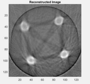
This week, we finally obtained a good reconstructed image from our scanner. The trick was adding the function fliplr! Below is our Matlab code and our reconstructed image.

Matlab code

% recon data from an ir ct scanner

%%%%%%%%%%%%%%%%%%%%%%%%%%%

% load the projection data

%%%%%%%%%%%%%%%%%%%%%%%%%%%

% full phantom data – acquired over 360 degrees of stepper motor

load ‘dataTEST_full.txt’; % data file you generate – needs to contain diodeVoltage, servoAngle, and stepAngle

diodeVoltage = dataTEST;

servoAngle = 40:1:128;

stepAngle = 0:1.8:269*1.8;

% %[row col] = size(data);

% outputflipped = zeros(270,89);

% % output = reshape(diodeVoltage, [271 89]);

% outputflipped(2:2:end,:) = fliplr(diodeVoltage(2:2:end,:));

% outputflipped(1:2:end,:) = diodeVoltage(1:2:end,:);

% %odd number rows

% %for ii = 1:2:col/2

%     %output(ii, 🙂 = diodeVoltage(ii, 1:col/2);

% %end

% 

% %even number rows

% for ii = 2:2:col/2

%     output(ii, 🙂 = fliplr(diodeVoltage(ii-1, 1+col/2:col));

% end

%%%%%%%%%%%%%%%%%%%%%%%%%%%

% recon parameters

%%%%%%%%%%%%%%%%%%%%%%%%%%%

N = 128; % matrix size

FOV = 12; % cm, FOV of image matrix

Dcm = 9; % cm, distance from fan beam vertex to center of stepper motor shaft

D = Dcm*N/FOV; % vertex->center distance in pixels

fanCenterAngle = 90; % fan center angle 

fanAngleWidth = 89; % total width we need in degrees for the fan beam to cover the object

%%%%%%%%%%%%%%%%%%%%%%%%%%%

% subtract off the center fan angle from the servo angles, to center them

%%%%%%%%%%%%%%%%%%%%%%%%%%%

servoAngle = servoAngle – fanCenterAngle;

%%%%%%%%%%%%%%%%%%%%%%%%%%%

% reshape data into a fan beam sinogram matrix. We assume that servo angle

% is minor dim in diodeVoltage vector

%%%%%%%%%%%%%%%%%%%%%%%%%%%

nServoAngles = length(unique(servoAngle));

nStepAngles = length(unique(stepAngle));

fanBeamData = diodeVoltage;

%fanBeamData = reshape(diodeVoltage,[nServoAngles,nStepAngles]);

%potVoltage = reshape(potVoltage,[nServoAngles,nStepAngles]);

%%%%%%%%%%%%%%%%%%%%%%%%%%%

% interpolate along the fan beam dimension to center the data

%%%%%%%%%%%%%%%%%%%%%%%%%%%

% find increment between servo Angles

deltaServoAngle = abs(diff(unique(servoAngle)));deltaServoAngle = deltaServoAngle(1);

% find increment between stepper motor angles

deltaStepAngle = abs(diff(unique(stepAngle)));deltaStepAngle = deltaStepAngle(1);

% get input (I) and output (O) interpolation grids

servoAnglesI = min(servoAngle):deltaServoAngle:max(servoAngle);

stepAngles = min(stepAngle):deltaStepAngle:max(stepAngle);

[stepAnglesI,servoAnglesI] = meshgrid(stepAngles,servoAnglesI);

servoAnglesO = -fanAngleWidth/2:fanAngleWidth/2;

stepAngles = min(stepAngle):deltaStepAngle:360-1.8;

[stepAnglesO,servoAnglesO] = meshgrid(stepAngles,servoAnglesO);

% do the 2D interpolation to the centered grid that we will use for recon

fanBeamDataCent = interp2(stepAnglesI, servoAnglesI, fanBeamData’, stepAnglesO, servoAnglesO, ‘cubic’, 0);

%servoAnglesI’, stepAnglesI’, fanBeamData,servoAnglesO’,stepAnglesO’,’cubic’,255);

%fanBeamDataCent(fanBeamDataCent > 100) = 255;

%sinogram

figure;imagesc(abs(fanBeamDataCent));

title(‘Sinogram’);

xlabel(‘Angle (degrees)’);

ylabel(‘Distance (cm)’);

colorbar 

%%%%%%%%%%%%%%%%%%%%%%%%%%%

% reconstruct the image

%%%%%%%%%%%%%%%%%%%%%%%%%%%

 img = ifanbeam(fliplr(fanBeamDataCent),D,’fancoverage’,’cycle’,’fanrotationincrement’,…

    deltaStepAngle,’fansensorgeometry’,’arc’,’fansensorspacing’,1,…

    ‘filter’,’Ram-Lak’,’frequencyscaling’,1,’interpolation’,’nearest’,…

    ‘outputsize’,N);

figure;imagesc(-img);axis image;colormap gray

title(‘Reconstructed Image’);

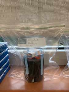
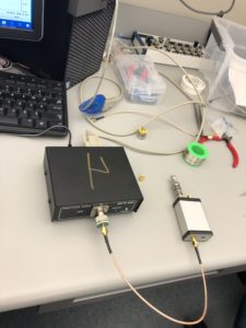
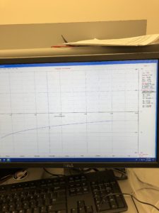
We also began to make our ultrasound scanner. We re-made the agar graphite phantom, since our phantom from last week separated into layers, and we soldered photodiodes, capacitors, inductors, and connectors onto our PCB board for the transmit/receive switch. Next, we used a windows software to  measure the power return loss of the switch. We found a 17 dB return loss. The set up of the T/R switch connected to the hardware and a screenshot of the frequency curve is shown below.

Question:

What values do you get for L and C?

L = 1.59  uH

C = 637 pF

Hunter Spivey and Aayush Gupta

This week we finished taking scans with our CT scanner and were able to characterize it’s performance on different phantoms and different settings of fan angle increments. We successfully reconstructed sinograms and images for these different cases, and finished our work with our IR CT. We also were able to make the mixture for the ultrasound phantoms and let it cure and solidify. Since we finished our phantom, we moved onto making our T/R switch for our ultrasound, and got a start soldering the components onto the switch itself.

Phantom 1: 1 Degree Increments

Phantom 1: 2 Degree Increments

Phantom 2: 1 Degree Increments

Hopefully next time we can finish our T/R switch and move onto the other parts of the ultrasound scanner if we have time.

Question:

What happens if you more coarsely or finely sample the fan beam angles?

Answer:

By doubling our fan rotation increment, and therefore cutting the number our projections in half, we noticed a significant drop in resolution of the final image. whereas before we could clearly distinguish the 8 different pegs, the more coarse acquisition was difficult to identify starting at the 6th largest peg. If you need to trade resolution for acquisition time however, and the loss of resolution isn’t important for your intended purpose, then it is a valuable method to increase acquisition speed.

Week 6

Javier and Nicholas J. Holden

Sadly, this is our last week looking and working with our homemade CT machine before we decided it needed to be destroyed. We ran our last data collection on several different phantoms for the report. We felt accomplished because we had tangible results. We tried to fully reconstruct the image but ran into some problems because the resulting image looked nothing like our phantom. After speaking with the Professor, we realized that we had incorrectly measured our dcm. Our previous thought was that it was the distance from the middle to the photodiode; however, it is the distance from the middle to the servo motor. We also played around with our servo center angle to try and correctly align our sinogram to the middle. Figure 1 demonstrates the finished sinogram. Notice how it is nicely aligned in the middle of the window. Figure 2 illustrates the reconstructed image of the phantom.

We also began our ultrasound lab. Our mold that was created last week turned out fantastic. The ice bath contributed to the success because of the lower temperature we were able to achieve before we stopped stirring. We also began to solder pieces to our electric board. I cannot begin to describe the frustration that Javier and I (Nicholas J. Holden) experienced when trying to solder the inductor to the board as it was a small and easily breakable component. Eventually, we were able to correctly solder it and were able to finish the TR switch. We still need to test the switch to ensure the TR switch is functioning like expected. 

Question: What values do you get for L and C? 

Answer: 1.59μH for the inductor and 636.5pF for the capacitor

Question: How close can you get to these values with the components we have (without, e.g. using multiple components in each position)?

Answer: We were able to get 1.5μH inductor and a 680pF capacitor.

Figure 1 – The sinogram

Figure 2 – Reconstructed image of our phantom

Antonio Glen, Hannah Kilpatrick and Danielle Liu

Update #5 Finishing the Infrared CT and starting Ultrasound

Last week, we continued to optimize our reconstruction. The final data set we made still resulted in a distorted reconstruction image, shown below. The sinogram for the data looked accurate, but was blurred around the edges. We believe slowing down the acquisition process in the future will all of to get a smoother sinogram and a more accurate reconstruction.

We also began to make agar phantoms for the ultrasound project. We mixed agar and graphite powder with water, microwaved the solution, and mixed it until it went down to 50 degrees Celsius. Then, we placed a 3D printed mold into the solution to finish making our phantom.

Questions

What parameters of your scanner and scan method influence resolution? Investigate these. 

The angle of the servo motor and speed of rotation.

Figure 1. Sinogram

Figure 2. Reconstructed image from sinogram

Week 5

Javier and Nicholas J. Holden

This week was spent focused on collecting and reconstructing the data. Luckily, our machine appeared to be functioning correctly, and no adjustments were needed to the machine.

We decided to collect data in two ways: two sweeps with our servo while our stepper is rotating at 60rpm and then one sweep with the servo. When there’s two sweeps, the ctRecon template image looks like a mirror image. Instead of trying to do some fancy math, we decided to collect the data in the two prescribed ways. It makes the math and future reconstruction a little easier.

We also changed the phantom to ensure that our code was running accurately and the data collected was changing with each phantom. Unfortunately, we experienced an issue with our servo / arm in that it could not move backward on the metal arm overhang. This meant we were not allowed to photo larger phantoms because there physically wasn’t enough space. The issue appeared to be that the person who configured the metal arm had hammered in a nut to a bolt and NOT a slider. Such brute force resulted in the slider unable to move backward. After an annoyed sigh, we decided to replace the phantom with a smaller one. While running the program on the replacement phantom, we made our own homemade auger phantom. To ensure we were protected from the graphite particulates and the Coronavirus, we wore masks. 

After microwaving the mixture, we had to continually stir it and wait for the temperature to decrease. Figure 1 illustrates this action by Javier. It was imperative that the two substances didn’t separate. We decided to create a bucket of ice to place the mixture in because we needed the auger/graphite mixture to reach a low enough temperature; this was important because we wanted to stop stirring while ensuring that there was minimal separation with the graphite and auger powder. As seen in Figure 2, we McGuyver’d the contraption. A dead battery was placed on top of the phantom in an effort to submerge it more into the liquid mixture. Afterwards, we placed tape everywhere and left it in a bag. We are excited to see what will happen to our device next week.

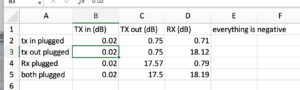
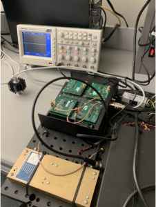
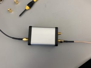
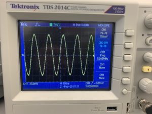
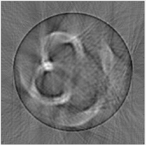
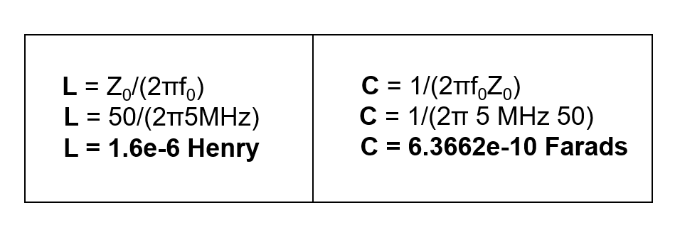
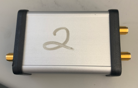
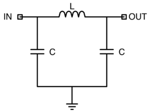
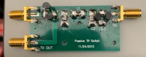
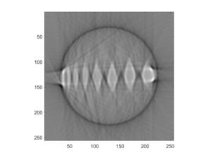
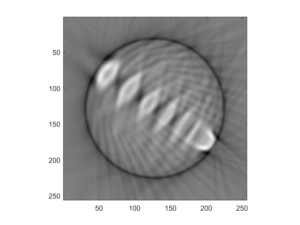
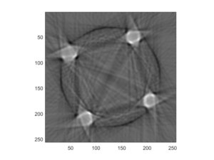
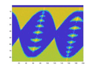
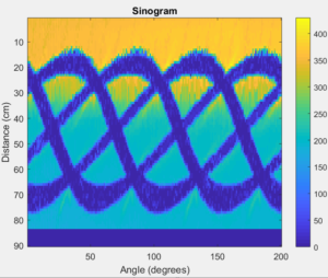
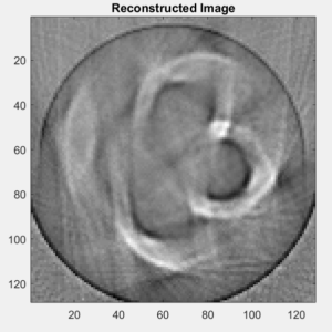
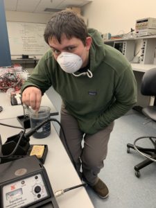
Figure 1 – Javier stirring the graphite/auger mixture

Figure 2 – The graphite/auger mixture inside a bag. The white dead battery is visible on top  of the orange phantom that was submerged into the liquid

Question: The servo has an extra (white) wire on it, that reads out its built-in position potentiometer, which you can use to record the servo’s actual position (rather than just its intended position). Is your image reconstruction improved by using this value instead of the intended value?

Answer: This would provide a more accurate measure of the servo angle but would require making sure that the servo is actually hitting all the positions in order to form the image. This may happen if there is something wrong with the servo and it is actually not hitting the right positions and would be visible with potentiometer voltages.