On Thin Ice
Posted by John Vrooman on Wednesday, May 8, 2019 in National Basketball Association, National Hockey League, Sports Econ Blog.
The big market clubs in NYC (MSG), LA (Staples) and Chicago (United) are noticeably absent from the NHL and NBA playoffs. Toronto Maple Leafs were knocked out in the first round of the playoffs and they haven’t won a Stanley Cup in 50 years.
Why are high revenue clubs not dominating the NBA and NHL as expected?
See 2018 NHL and NBA Team Values.
Asymmetric Markets
On the demand side, most professional sports clubs have local monopolies (only one seller) in their respective home product markets (gate, venue and local media revenues), because multiple team product markets are inferior negative-sum moves in league expansion. Existing multiple team markets are usually the post-facto result of rival league mergers in the past. (See the dual market theorem.)
On the supply side, competing sports clubs are usually assumed to be passive “price takers” in a competitive labor market because no club has the power to set the market clearing free-agent rate. In this case the profit maximizing large market club would dominate the small market club by roughly the same ratio as their market sizes.
QFV Profit-Max Theory
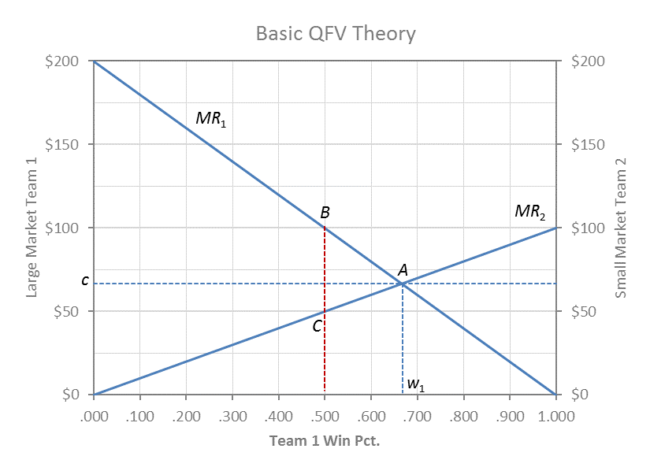
In the QFV graph above, the large market club (MR1 moving left to right) is twice the size of the small market club (MR2 moving right to left) and the profit max equilibrium would be point A, where w1 = .667 and w2 = (1 – w1) = .333.
If the league was evenly matched at .500, team 1 at B could outbid team 2 for talent at B (MR1 > MR2) and improve toward A. If the league was dominated by team 1 to the right of A, then team 2 could actually outbid team 1 (MR2 > MR1) and improve to the left toward A.
MR1 is the derivative of the revenue function for team 1 and the curve slopes downward because of diminishing marginal revenue for winning (fans prefer winning competitive games rather than blowout after blowout).
Revenue for team 1 in league equilibrium would then be the area of the trapezoid under MR1 to the left of w1, and the trapezoidal area under MR2 to the right of w1 = (1 – w2) is the revenue for team 2.
The market clearing (equilibrium) wage rate would be c per win (WAR) = MR1 = MR2 for both clubs, and the relative payrolls would be the (2/1) rectangles bounded by c and w1/w2 = 2/1.
The respective profit margins are the areas of the respective triangles between each team’s MR and its team payroll. The rate of talent exploitation is zero because players are paid (c) their MR (marginal revenue product) at A where c = MR1 = MR2.
Monopsony Power
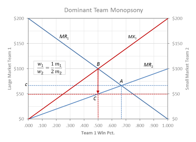
If the large market club had dominant monopsony (one buyer) power in the labor market to set the wage rate, then it would lay back and maximize profit by not paying any more for talent than the maximum small market team would pay along MR2. A monopsony club would only have to match the best offer at C from team 2.
In the monopsony case the league profit-max equilibrium would be at B and the players would only be paid the wage rate $50 at point C. Team 1 would maximize profit by exploiting talent at C on MR2 when talent is really worth MR1 at B.
The monopsony profit max condition shown in the above graph (m1/m2 = 2) would result in a 50/50 league balance in winning and relative payrolls. w1/w2 = 1/2 m1/m2 = 1.
Revenues are the trapezoidal areas under the 2 respective MR curves and profits are the areas between the respective MR curves and the team payrolls.
In monopsony labor theory MX1 is the dominant team’s “marginal expenditure” curve and MR2 serves as the labor supply curve for Team 1 (MX1 = 2 MR2). Profits for the dominant monopsony Team 1 are maximized at point B where MR1 = MX1.
Salary Cap
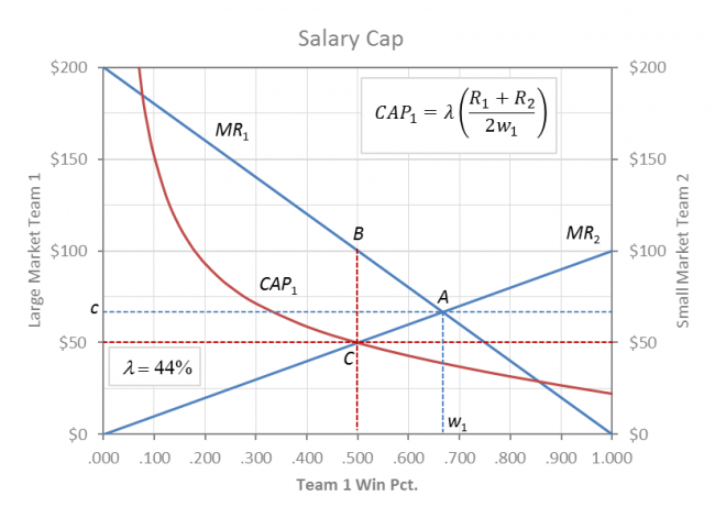
Both teams are better off in a balanced league (w1 = w2), because their mutual profits are derived from the exploitation of talent (c < MR). The hard salary cap (set at 44% of league revenues in this case) in the above graph is an effective profit-max instrument that ensures the monopsony club’s exploitative (c < MR) solution at point C.
Team 1 cannot take its payroll above the CAP1 contour and so the constrained league equilibrium lies at the intersection of CAP1 and MR2 at C. Player payroll decreases by the rectangle c – $50 and the profit exploitation gains are split evenly between the clubs.
Under dominant team 1 monopsony profits increase for both clubs, but total league revenue and social welfare are actually decreased by the area of the lost triangle ABC. Team 2’s revenue gain at .500 is more than offset by the decline in revenue for team 1.
In this respect a dominant monopsony salary cap is welfare inferior because team 1 has more excluded fans who are willing to pay more for large market team 1 to win than small market team 2, and profit increases are derived from player exploitation c < MR1 at C.
Revenue Sharing Paradox
Intuition suggests that the more random outcomes in the NHL are perhaps associated with competitive balance engineering through increased revenue sharing. This would be true if owners are sportsmen who spend all their revenue on talent, but if owners are profit maximizers then this is not the case.
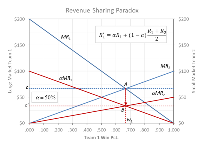
Most revenue sharing schemes are pool-sharing formulas (like the one in the graph) where the home team keeps a percentage α of local revenue (first term in graph) and contributes the visitors’ share (1 – α) to a pool that is then split equally among the rest of the league (second term in graph). The advantage of pooled sharing is that it equalizes the visitors’ share across the rest of the league.
As the home-team share decreases, the economic incentive to win simultaneously decreases proportionately among all teams by the proportion of local revenue that is shared (taxed). In the above graph the MR curves shift downward in the same visitors’ share proportion for both clubs.
The league equilibrium shifts from A to B where the balance between teams remains the same as without revenue sharing, but the going wage rate drops from c to c’ by the percentage of revenue that is shared, (1 – α) = 50% in this case.
This leads to the invariance proposition: Competitive balance remains unchanged by revenue sharing, but the degree of exploitation of talent increases by the amount of revenue that is shared (1 – α). More advanced analysis later shows that revenue sharing actually leads to less balance for profit maximizing teams.
The paradoxical result is best explained by viewing revenue sharing an instrument of progressive product market cartelization of seemingly competitive clubs in the monopoly league-cartel. The amount of revenue shared (1 – α) serves as an index of the degree of cartelization in a monopoly sports league cartel.
In the graph the revenues of the two clubs are the home-team α-share areas under their respective MR’ curves, plus the total area between both MR and MR’ curves split equally between the clubs as their visitors’ share. Profits are each team’s revenues minus their respective payrolls that are progressively shrinking under c’.
At the α=0 revenue sharing limit, the players share has been reduced to their reservation wage c’ = αc →0 and the league has become a perfectly syndicated cartel where all teams have an equal revenue share, (R1 + R2) / 2.
As α→0 payrolls sink to a minor league level (reservation wage), both teams benefit from large-market dominance and the cartel’s joint profit maximum objective is the same as revenue max at w1/w2 = 2/1.
When revenue sharing and salary cap are combined (NFL), revenue sharing progressively defeats the cap as α→0 and ultimately competitive balance decreases from .500 back to w1 = .667.
If the cap has also has a minimum (NFL, NBA and NHL) then α→0 would ultimately lead back to absolute balance at .500, where both profit max clubs would have the same payrolls at the salary minimum.
If the owners are win-maximizing sportsmen then all revenues would be spent on talent. In this case profit margins would be zero, and the large market club would totally dominate the smaller club 1.000/.000. Revenue sharing and/or salary caps could reverse engineer the optimal competitive balance.
Big 4 revenue sharing comparisons.
For full development of QFV Theory see Two to Tango.
©2024 Vanderbilt University · John Vrooman
Site Development: University Web Communications