Revenue Sharing: Quest for Certainty
Posted by John Vrooman on Thursday, June 11, 2020 in Major League Baseball, National Basketball Association, National Football League, National Hockey League, Sports Econ Blog.
“We (NFL owners) are a bunch of fat-cat Republicans who vote socialist on football.”
—Art Modell, former owner of the NFL Cleveland Browns/Baltimore Ravens
“The NFL is a perfect portfolio.”
—John Vrooman, The Economist
League Think
Over the last half-century the NFL has become the most economically powerful sports league in the world largely because it has also been the most egalitarian. In 2019 NFL clubs pool-shared $8.8 billion (60 percent) of a total $14.5 billion in revenues among its 32 franchises.
The underlying source of NFL economic strength has been a survivalist “league-think” mentality that developed during inter-league competition of the NFL-AFL rival-league war 1960–1966. League-think is the collectivist notion that any sports league was only as strong as its weakest franchise.
Evenly shared national media money has grown at an exponential rate of 12% from $47 million annually at the time of the actual AFL-NFL merger in 1970 to $6.68 billion per season under the current 2014–2021 TV rights contracts (B4 TV rights). (Local media revenue is insignificant in the NFL.)
The source of the sports media explosion was the Sports Broadcasting Act of 1961 in which the US Congress granted sports leagues monopoly-cartel power in negotiating TV deals. The underlying justification was that sports leagues are natural cartels and that league parity is welfare superior because of the joint-production of the games,
The SBA assumed that economic disparity created by asymmetric media market size translated directly to on-field disparity among teams that damaged fan welfare. Competitive balance derived from collective media rights negotiation was justified as being be fan-welfare superior, a priori.
Over the last quarter century a major threat to old-school league-think solidarity has emerged from an individualist counterrevolution in venue revenue (concessions, parking, sponsorships and luxury seating) that is sheltered from sharing with the rest of the league.
During the luxury-seat stadium building frenzy that followed the watershed 1993 Collective Bargaining Agreement (CBA), the proportion of tax-sheltered team-specific venue revenues doubled from 10% to 20% of total revenues. (NFL gate revenue is also 20 percent of the total and pool-shared 66% home/34% visitor).
This once-tight NFL syndicate is now split into those nouveau-riche teams with new tax-payer funded cash-cow venues sheltered from revenue sharing, and those without. (Cowboy Capitalism)
The underlying objective in the economic theory of a firm is for franchise owners to maximize profit π = R-C (revenue – cost), but the more realistic financial goal is to maximize franchise value V = π/r, where r is a risk-adjusted discount rate.
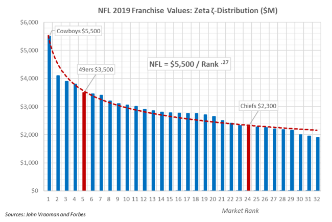
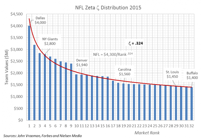
The graph above shows NFL franchises ranked in order of declining franchise value with the most valuable Dallas Cowboys ranked first in 2019 at $5.5 billion and the Buffalo Bills ranked 32nd at $1.9 billion. The two 2020 Super Bowl teams (SF 49ers and Champion KC Chiefs) are shown in red.
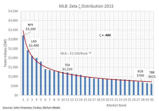
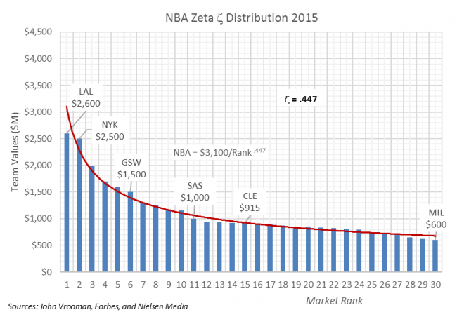
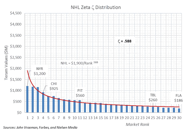
The value-rank equation V = $5.5b / Rank^ζ, measures the rate of value decline, left to right from most valuable to least valuable franchise. The zeta exponent ζ ranges from zero to one, where ζ = 0 implies absolute equality among teams and ζ = 1 generalizes Zipf’s Law as a special ζ-case, where a team’s value equals the highest team’s value divided by that teams rank: V = V1/Rank.
Zeta ζ-indexes are shown below for the Big 4 leagues and the underlying TV-market size distribution for the 2019 season. The NFL clearly has the most equitable distribution of franchise worth with ζ = .271 as it improves the underlying imbalance in TVHH market size ζ = .551 by 50 percent.
The NBA is the (distant) second most balanced in franchise value, followed by MLB and the least balanced NHL, but all leagues improve on the underlying difference in TV household market-size.
| 2019 | FLAT | NFL | NBA | MLB | NHL | TVHH | Zipf |
| Zeta | .000 | .271 | .422 | .471 | .496 | .551 | 1.000 |
These results are consistent with the 2019 team-value and revenue ratios of the top 10 clubs to the bottom 10 clubs in the Big 4 NA leagues shown below, with the order of MLB and NHL reversed. These distributions accurately reflect the approximate home/league revenue splits for the Big 4 leagues: NFL 40%/60%; MLB and NBA 50%/50% and NHL 60%/40%,
Top 10/Bottom 10 Ratios 2019 ($M) |
||||
| MLB | NFL | NBA | NHL | |
| Value | ||||
| Top 10 | $2,713 | $3,700 | $3,168 | $1,057 |
| Bottom 10 | $1,119 | $2,153 | $1,451 | $454 |
| Value Ratio | 2.43 | 1.72 | 2.18 | 2.33 |
| Revenue | ||||
| Top 10 | $258 | $402 | $247 | $139 |
| Bottom 10 | $440 | $536 | $353 | $211 |
| Revenue Ratio | 1.71 | 1.33 | 1.43 | 1.52 |
| Source: John Vrooman and Forbes. Net revenue after revenue-sharing “taxes”. | ||||
In the economic theory of sports leagues there are two inter-related optimization problems.The first is competitive team owners an seeking internal profit maximum and the second is the impact of profit seeking on an external social welfare optimum for owners, fans, and players.
In theory, the spirited competition among teams and leagues drives the pursuit of internal profit by owners toward the external social optimum. In a perfectly competitive market there are no excess profits for owners, fans pay a fair price to see their home team win close games and players are paid what they are worth.
Unfortunately in the real world of negative-sum monopoly and monopsony cartel power of sports teams and leagues, the pursuit of the internal optimum by owners precludes the satisfaction of the external optimum for everybody else.
Monopoly cartels are groups of potentially competing firms that collude to act as one monopoly and charge fewer fans more than they would otherwise pay and pay fewer players less than they would otherwise earn in an open competitive market.
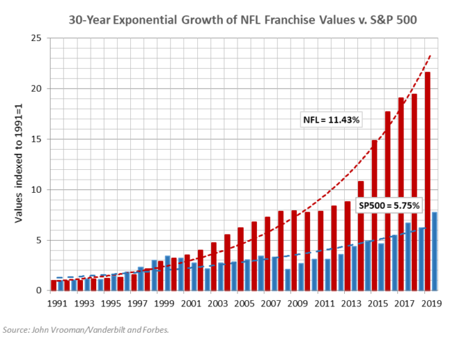
The graph above compares the 11.4% exponential growth in NFL franchise values to the 5.75% growth in the S&P 500 stock index over the last 30 years. The fact that NFL value growth more than doubles that of the most competitive open-market rate is prima facie proof of the unregulated monopoly and monopsony power of the NFL cartel.
The same is true for exponential growth in the other 3 major NA professional sports league cartels over the same period: MLB and NBA = 9.5% and the NHL = 8.5%.
Risky Business
Like any financial asset, the base value of a sports franchise is equivalent to the risk adjusted present value (PV) of the discounted (foregone interest rate r) net cash flow (CF) derived from that franchise (asset).
For a given future year t, PV = CF/(1+r)^t and for multiple future years t = 1 through n, PV = ∑ (t=1,n) CF/(1+r)^t.
As n approaches perpetuity, then PV → CF/r = CF/(r* + ε), where the discount rate r is equal to the risk-free market interest rate r* adjusted for risk ε, such that r = r* + ε. Projected growth in cash flow can also be captured by subtracting the anticipated growth rate γ from the risk-adjusted discount rate RADR: r = r* + ε – γ. The cash-flow valuation multiple is simply μ = 1/r.
The valuation math of a sports franchise is straightforward. For example, if the average NFL club is worth $3 billion with net cash flow of $300 million, then that implies a cash-flow valuation multiple of μ =10 and a risk adjusted discount rate of 10% (μ = 1/r = 1/10%).
So if the risk-free market rate on 3-month T-Bills is r*= 2%, then the risk adjustment factor in this case is ε = 10% – 2% = 8%. As the cash flow becomes more uncertain, the risk factor ε increases and franchise cash flow becomes less valuable.
In the inherently risky business of professional sports, the subjective estimation of ε is critical to financial decisions. At some point the elimination of projected risk becomes just as, if not more important than increasing the volume of net cash flow. Big-league cartel owners often trade the maybe for the sure cash flow in maximizing their franchise values.
The chart below uses the values and revenues estimates by Forbes to derive hypothetical discount rates for the Big 4 NA professional sports leagues. The cash-flow valuation multiple μ roughly equals twice the Value/Revenue ratio, because payroll costs are about one-half of revenues in all leagues.
Cash flow is more precisely estimated as Revenue-Players Share and μ = Value/CF. This implies that RADR = 1/μ. Franchise value can be increased by increasing revenues, reducing player costs share or decreasing the uncertainty of both positive and negative elements of net cash flow.
This valuation method assumes competitive capital markets. So it is important to realize that franchise values shown below systematically underestimate the auction selling price for a rarely available monopoly sports franchise by about 20%-25%. (See Winner’s Curse and Basketball Jones.)
Risk Adjusted Discount Rates
| NFL | MLB | NBA | NHL | |
| Avg Value | $2,855.2 | $1,776.0 | $2,123.0 | $667.0 |
| Revenue | $452.4 | $329.8 | $292.0 | $164.1 |
| V/R | 6.31 | 5.38 | 7.27 | 4.07 |
| Payroll/R | 48.6% | 46.9% | 45.1% | 48.1% |
| Cash Flow | $232.4 | $175.2 | $160.2 | $85.2 |
| CF/R | 51.4% | 53.1% | 54.9% | 51.9% |
| Profit/R | 22.6% | 12.0% | 24.0% | 15.3% |
| μ-Multiple | 12.28 | 10.14 | 13.25 | 7.83 |
| RADR = r | 8.1% | 9.9% | 7.5% | 12.8% |
| Source: John Vrooman and Forbes | ||||
Modern portfolio theory (mean-variance analysis) is a mathematical model where the expected return Rp of a portfolio of assets is maximized for a given level of risk σp. It provides an argument for diversification in investing, where overall portfolio risk can be reduced by investing in combinations of assets that are not perfectly positively correlated (-1 ≤ ρ < 1), where ρ is a correlation coefficient among asset returns.
Portfolio return is the weighted combination of the component asset returns and portfolio volatility (variance) is a function of the correlations ρ of the component assets. Minimum risk reduction (zero) occurs when the correlation among assets is perfectly positive ρ = 1 and maximum risk reduction results from combining assets with a perfectly negative correlation ρ = -1. An effective diversification strategy simply combines uncorrelated assets, and a perfectly diversified zero-risk portfolio combines assets with a perfectly negatively correlation.
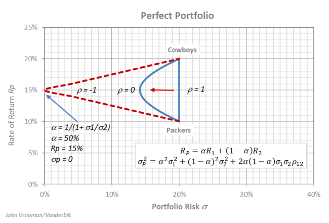
The graph below shows a sports league in risk-return space as a natural revenue-sharing portfolio with perfectly negative win-loss correlation between 2 teams. Given the zero-sum nature of the volatility of teams within a closed league, revenue sharing can create team-specific value by reducing risk.
This is true for teams with different expected rates of return and risk, teams with different rates of return and the same level of risk and similar teams with identical rates of return and risk. Sports leagues are a natural for risk minimization through diversification by the unique virtue of teams sharing revenue with opponents that have exactly the opposite fortunes, ρ = -1.
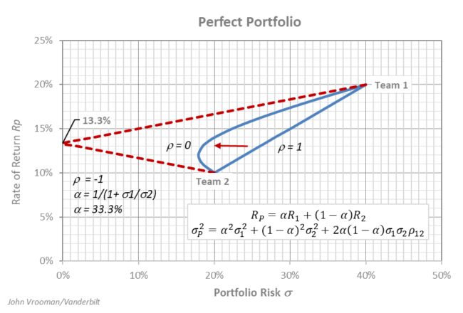
In isolation, Team 1 has an expected return of R1 = 20%, but a relatively risky standard deviation of σ = 40%. By comparison Team 2 has a lower expected return of R2 = 10% that carries less risk at σ = 20%. In league portfolio combination the expected return Rp is simply the linear average of R1 and R2 weighted by the revenue sharing proportion: Rp = αR1 + (1-α)R2, where 0 ≤ α ≤ 1.
If the financial performances of the two clubs are perfectly correlated ρ = 1, then the league portfolio also carries the weighted average risk of the two teams: σp = ασ1 + (1-α)σ2. In this extreme case there is no objective diversification advantage along the linear risk-return combination of the two teams. (See table below.)
The appropriate revenue-sharing proportion chosen along that frontier depends solely on the subjective risk-return preferences of the team owners who rationally prefer to head northwest in risk-return space seeking the best available combination of high return and low risk for their clubs.
If the teams’ performances are perfectly negatively correlated ρ = -1, then league portfolio diversification creates the objective possibility of a minimum risk portfolio of zero of the for the league: σp = ασ1 – (1-α)σ2.
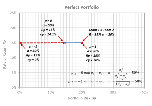
A revenue sharing league could objectively have an expected return of Rp = 13.3% with zero risk σp = 0 if α* = 33.3%. More generally, a zero-sum sports league (ρ = -1) can achieve minimum zero-risk diversification when α* = σ2 / (σ1 + σ2). (See table below.)
The risk-return preference is still subjective depending on the owners but now it lies on the superior choice set along the linear frontier between Team 1 and the zero-risk choice.This is because any choice along the lower linear combination would be inferior to the upper frontier in terms of league risk-reward.
Even if the correlation is not perfectly positive or negative (-1 < ρ < 1) revenue-sharing diversification can still objectively improve the risk-reward choice set. For example, if ρ = 0 a minimum portfolio risk choice exists at the vertex of the parabola shown in the graph.
This league could set α* = 20.0% and choose a return of Rp = 12.0% with minimum risk σp = 17.9% . More generally, if ρ = 0 a league can achieve minimum risk diversification when α* = σ2^2 / (σ1^2 + σ2^2). (See table below.)
Minimum Risk Portfolio
(R-return, σ-risk): Team 1 (20%, 40%) vs. Team 2 (10%, 20%)
| α | 1-α | Rp | Portfolio Risk σp | ||
| ρ = 1 | ρ = 0 | ρ= -1 | |||
| 0% | 100% | 10.0% | 20.0% | 20.0% | 20.0% |
| 10% | 90% | 11.0% | 22.0% | 18.4% | 14.0% |
| 20% | 80% | 12.0% | 24.0% | 17.9% | 8.0% |
| 30% | 70% | 13.0% | 26.0% | 18.4% | 2.0% |
| 33% | 67% | 13.3% | 26.7% | 18.9% | 0.0% |
| 40% | 60% | 14.0% | 28.0% | 20.0% | 4.0% |
| 50% | 50% | 15.0% | 30.0% | 22.4% | 10.0% |
| 60% | 40% | 16.0% | 32.0% | 25.3% | 16.0% |
| 70% | 30% | 17.0% | 34.0% | 28.6% | 22.0% |
| 80% | 20% | 18.0% | 36.0% | 32.2% | 28.0% |
| 90% | 10% | 19.0% | 38.0% | 36.1% | 34.0% |
| 100% | 0% | 20.0% | 40.0% | 40.0% | 40.0% |
| John Vrooman /Vanderbilt University | |||||
Competitive League
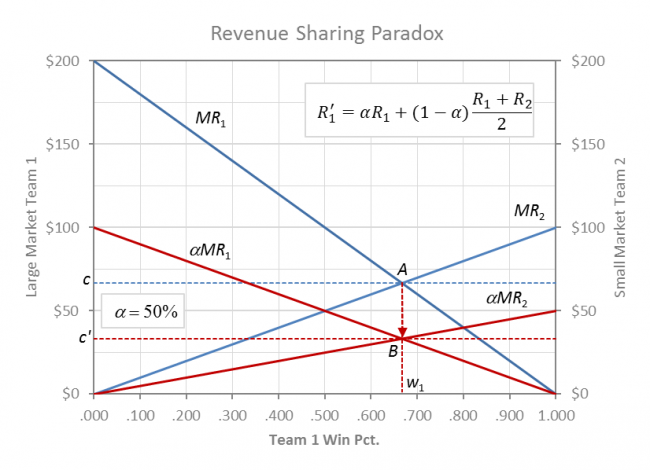
The economic effects of revenue sharing on competitive balance and the two optima can be visualized in the above graph of the comparative marginal revenue of winning for two-teams in a zero-sum league with asymmetric market size.
Team 1’s market is shown as twice the size as team 2 on the vertical axes, and the negatively sloped curves reflect diminishing marginal returns to winning for fans of both clubs. MR is the slope (derivative) of a revenue function with a decreasingly positive slope. Additional wins are worth progressively less to fans because they prefer defeating quality opposition by a close margin (competitive balance).
A large market team 1 moves horizontally from left to right as it wins games by acquiring talent from team 2. Small market team 2 moves from right to left as it competes head to head with team 1 for talent and wins.The zero-sum nature of a game implies that w2 = 1 – w1 along the horizontal axis.
The MR curves are the demand curves for talent for each of the two teams, where players are paid their value to the team with the higher MR. If MR1 > MR2 then team 1 will acquire talent from team 2 and the w1 will move to the right. If MR2 > MR1 then reverse is true for team2, and w2 will move to the left.
Competitive league equilibrium is shown in the graph at point A where w1 = .667, w2 = .333 and the market wage rate is c = MR1 = MR2 = .667. More generally, competitive balance at league equilibrium is the ratio of market size w1/w2 = m1/m2.
Visually total revenue for team 1 is the trapezoidal area under the MR1 curve to the left of w1 = .667 and total revenue for team 2 is the area under MR2 to the right of w2 = .333. Total payroll for team 1 is the rectangular area under c to the left of w1 and total payroll for team 2 is the area under c to the right of w2. Profit for either team is the triangular difference between the revenue areas under each of their MR curves and respective team payrolls.
The pool-sharing formula used by all Big 4 leagues is shown for α = 50%, where MR1′ = αMR1 + (1-α)(MR1 + MR2)/2 and MR2′ = αMR2 + (1-α)(MR1 + MR2)/2. Team 1 retains an α-share of its home revenue (50%) and contributes an (1 – α) share (50%) to a pool that is redistributed equally to all teams, regardless if they win or lose. Above average revenue teams are net payers and below average revenue teams are net recipients of pooled revenue sharing.
The effects of revenue sharing on competitive balance are shown as both opposing MR curves shifting downward by the amount of revenue that is shared (1-α). If revenue sharing formulas are symmetrical then both curves shift downward by the same proportion, because the value of winning has been proportionally reduced for both clubs. As the teams share revenue the league solution also shifts downward from A to B by the (1-α) percentage of revenue that is shared.
The paradox of revenue sharing is that at the new league equilibrium B, competitive balance remains unchanged (Invariance Proposition) from point A. The major difference is that all playing talent is now exploited because at equilibrium B, players are paid (1-α) less (50%) than their marginal revenue at A (αc = αMR < MR). (The invariance proposition holds for revenue sharing in combination with salary caps, but it does not hold if owners are sportsman rather than profit maximizers. See Two to Tango).
With pooled sharing the clubs retain home revenues under the respective αMR curves and essentially split the combined areas between the MR curves and αMR curves. Small market team 2 benefits clearly from sharing as they are trading a share of m2 revenue for m1 revenue (R1 > R2). Revenue sharing also increases profit for the large market club through the exploitation of talent.
Although large market team 1 losses revenue in the swap, they benefit profit-wise because the gains from the exploitation in talent (1-α)c more than compensate for the loss of the net revenue sharing transfer payment (1-α)(R1 – R2)/2.
| α | w1 | w2 | R1 | R2 | Transfer | c | C1 | C2 | π1 | π2 |
| 100% | .667 | .333 | .888 | .277 | .000 | .667 | .444 | .222 | .444 | .055 |
| 50% | .667 | .333 | .736 | .430 | .153 | .333 | .222 | .111 | .514 | .319 |
| 0% | .667 | .333 | .583 | .583 | .306 | .000 | .000 | .000 | .583 | .583 |
As revenue sharing increases α→0 the rate of exploitation also increases as the two competitive teams effectively collude and morph into a monopoly/monopsony league cartel that maximizes total league revenue and joint profit. Maximum league revenue and joint profit also occurs at w1/w2 = .667/.333. The (1-α) league-share measures the rate of talent exploitation, and serves as an index of monopsony cartelization for the league (one-buyer of talent).
This answers the common anti-trust legal question about whether a league is the firm or a group of separate competitive firms (Section 1 v. 2 of the Sherman Act). The rule of reason answer is both. Monopoly cartelization in a sports league is a matter of degree depending on the amount of revenue that is shared. At the limit as α→0, the league becomes a single-entity monopoly firm.
Squeeze Play
The relatively recent luxury stadium counter-revolution by a new breed of maverick owners to avoid the revenue sharing “tax” is also driven by a quest for certainty. In single pursuit of the internal optimum, individual franchises sacrifice the external social optimum as value-maximizing owners shift franchise-specific performance risk to the home-town season-ticket holders.
Teams can mutually avoid risk by portfolio revenue sharing, but they also can reduce risk in un-shared local revenue through price discrimination. The first method increases value by reducing risk at the expense of the players (exploitation), and the second method reduces fan welfare.
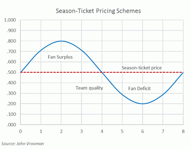
Season tickets extract the consumer surplus (market prices are lower than high-demand fans would pay) through all-or-nothing pricing. A uniform season price is charged for both high demand games and low-demand games.Season-ticket fans will be forced to pay more than they want for low demand games (fan deficit) in order to enjoy high demand games for less than they would be willing to pay (fan surplus). Season prices are set so that fan surplus = fan deficit.
Season tickets also carry an option for post-season tickets and the option to renew. Season tickets are implicit quasi-contracts where season-ticket holders agree to endure bad games and losing seasons in order to get tickets for the high demand events. In doing so, the season ticket base has assumed all risk inherent in the team talent cycles of winning and losing (tanking) and the owners have insured a relatively certain quasi-contractual cash flow upfront.
In leagues with excess demand created from shorter seasons (NFL) upfront PSL (personal seat license) payments are usually required for all season tickets. If properly set a PSL price is the present value of a season ticket discount through time.
For example, a season ticket price of $1000 is equivalent to a discounted ticket price of $500 that carries an up-front PSL payment of $5000 (PSL = $500/r assumes r = 10%). If perpetual PSLs have time limits or insufficient season-price discounts, then they will usually go unsold. Once again the owners capture the certain cash flow upfront, while the loyal fan base assumes the performance risk throughout the cycle.
Teams in leagues with longer winning elastic seasons use variable pricing techniques instead of PSLs to complement their partial season-ticket sales. Almost all NFL (8 home games) tickets are season tickets, while the other 3 leagues (MLB 81 home games, NBA and NHL 41 games at home) have season-ticket bases slightly over 50% of the total tickets, on average.
PSLs work best in the sold-out excess-demand NFL while the other leagues discriminate (capture the fan surplus) using variable pricing schemes where the primary market prices (sold directly by the team) match the quality of the games and mimic resale prices in the secondary market. Team owners can flatten their inherently cyclical team-performance risk curves.
During the luxury venue counter-revolution, publicly funded multipurpose cookie cutter stadiums were replaced by smaller more exclusive single-purpose venues to maximize profit, reduce risk and create franchise value (internal profit max optimum).The expansive multipurpose cookie cutters had been designed to maximize fan welfare allowing all fans to watch games at the lowest possible uniform price (external social welfare optimum).
The prototypical inside-out of the new venue design was a revolutionary form of spatial price discrimination where lower bowl and upper-deck seating are attached to a luxury-seat motel in the middle, rather than the inverse in the cookie cutters. Using a classic monopoly tactic, fans are charged higher luxury seat prices, and marginal fans are excluded by price.

The cross-section of a typical venue design is shown above comparing a proposed LA Coliseum before and after renovation.The core structure is a luxury motel comprised of a mezzanine of club seats with rows of luxury suites above and below.
Contractually obligated venue revenues from club seat fees and luxury-suite leases are excluded from the revenue-sharing base.The new venues are profit-maximizing cash-cows but they are also part of a broader squeeze play that shifts inherent performance risk from the teams to their fans.Teams increase franchise value by trading the maybe for the sure, because a bird in the hand is worth two in the bush. According to the law of conservation of risk however, the exclusive fan base pays the full price. V↑ = π↑ / r↓
Appendix A: Perfect Portfolios
Equal-Risk Portfolio
(R-return, σ-risk): Team 1 (20%, 20%) vs. Team 2 (10%, 20%)
| α | 1-α | Rp | Risk σp | ||
| ρ = 1 | ρ = 0 | ρ = -1 | |||
| 0% | 100% | 10.0% | 20.0% | 20.0% | 20.0% |
| 10% | 90% | 11.0% | 20.0% | 18.1% | 16.0% |
| 20% | 80% | 12.0% | 20.0% | 16.5% | 12.0% |
| 30% | 70% | 13.0% | 20.0% | 15.2% | 8.0% |
| 33% | 67% | 13.3% | 20.0% | 14.9% | 6.7% |
| 40% | 60% | 14.0% | 20.0% | 14.4% | 4.0% |
| 50% | 50% | 15.0% | 20.0% | 14.1% | 0.0% |
| 60% | 40% | 16.0% | 20.0% | 14.4% | 4.0% |
| 70% | 30% | 17.0% | 20.0% | 15.2% | 8.0% |
| 80% | 20% | 18.0% | 20.0% | 16.5% | 12.0% |
| 90% | 10% | 19.0% | 20.0% | 18.1% | 16.0% |
| 100% | 0% | 20.0% | 20.0% | 20.0% | 20.0% |
| John Vrooman /Vanderbilt University | |||||
Equal-Team Portfolio
(R-return, σ-risk): Team 1 = Team 2 = (15%, 20%)
NFL Portfolio Finance 2019 ($M) |
|||
| Team | Cowboys | NFL Avg. | Packers |
| Value | $5,500.0 | $2,855.2 | $2,850.0 |
| Revenue | $950.0 | $452.4 | $456.0 |
| National | $274.3 | $274.3 | $274.3 |
| Local | $675.7 | $178.1 | $181.7 |
| Gate | $108.0 | $70.0 | $74.0 |
| Player | $190.0 | $219.9 | $245.0 |
| Profit | $420.0 | $102.1 | $39.0 |
| Value/Revenue | 5.79 | 6.31 | 6.25 |
| National % | 28.9% | 60.6% | 60.2% |
| Local % | 71.1% | 39.4% | 39.8% |
| Gate % | 11.4% | 15.5% | 16.2% |
| Players % | 20.0% | 48.6% | 53.7% |
| Profit % | 44.2% | 22.6% | 8.6% |
| John Vrooman /Vanderbilt | |||
Appendix B: Zipf and Zeta
©2024 Vanderbilt University · John Vrooman
Site Development: University Web Communications