Salary Cap: Monopsony Power Play
Posted by John Vrooman on Thursday, April 23, 2020 in Major League Baseball, National Basketball Association, National Football League, National Hockey League, Sports Econ Blog.
Salary Cap Theory / Big 4 Cap History / Cap Graphs / Combo Graphs / Cap Mechanics / QFV Theory / CBI & Beta Balance / Perfect Game / Two to Tango / Monopsony Power /
“In theory there is no difference between theory and practice. In practice there is.”
–Yogi Berra
Quid Pro Quo
Salary caps in professional sports originated in the 1984-85 season when the NBA sought to limit rapidly rising payrolls associated with the restricted free-agency granted to veteran players in the 1976 CBA as part of the Oscar Robertson free-agency settlement. The NBA cap is a “soft cap” in that it can be avoided through a number of exceptions that favor dominant teams in their attempts to re-sign their own free agents. The most notable was the Larry Bird free-agent exception for the Boston Celtics during the league-saving “Magic vs. Bird” Lakers-Celtics rivalry that ran throughout the 1980’s.
A decade later, a hard (unavoidable) salary cap was imposed in the NFL in 1994 to negate the salary effects of the free-agency of NFL players granted in the 1993 CBA as part of the Freeman-McNeil free agency settlement in 1992. A decade after that the NHL owners imposed a hard cap in the 2006 CBA after the 2004-05 lockout. Salary caps have emerged as a constant “quid pro quo” countervailing companion to the free agency of players.
The relatively strong MLBPA had also obtained free agency in its 1976 CBA, and the players’ union had frustrated MLB owners’ attempts to impose a salary cap before, during and after the 1994-95 strike.
NBA veteran players had successfully avoided the hardening of the avoidable soft cap in the 1998-99 lockout, but a poison pill luxury tax (labeled a competitive balance tax in MLB) was inserted into both MLB (2002) and NBA (1999) turn-of-the-Century CBAs.
The relative strength of a sports union is a function of the average career length of its players (shorter = weaker), and reflected in the length of their current CBAs. (Shorter = stronger: MLB = 5 yrs, NBA = 7, NFL and NHL = 10 yrs.) See the GRID.
By 2003 both MLB and the NBA (2002-03) implemented luxury tax rates and surcharges that would become so progressively restrictive that both leagues had imposed de-facto hard salary caps that limited salary growth for free agents.
In theory, the salary cap works to prevent large-market teams from signing the best free agents from smaller market clubs. It is argued that small market teams under the cap could sign free agents and improve their chances of winning.
In reality, the salary cap doesn’t help the weak teams so much as it prevents wealthy teams from competing for each other’s players. The end result has become profit maximizing random mediocrity through monopsony cartel talent exploitation disguised as fair-play and competitive balance.
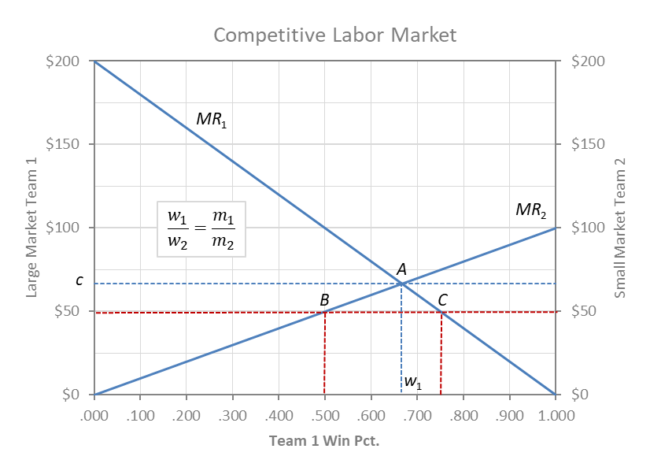
Competitive Labor Market
The graph above shows the marginal revenue of winning for two-teams in a zero-sum two-team league with asymmetric market size. Large market team 1 moves horizontally from left to right as it wins by acquiring talent and small market team 2 moves from right to left as it competes head to head with team 1 for talent and wins.The zero-sum nature of winning and losing means that w2 = 1 – w1 along the horizontal axis.
Team 1’s market is shown as twice the size as team 2 on the vertical axis, and the negatively sloped curves reflect diminishing marginal returns to winning for the fans of both clubs. MR is the slope or derivative of a parabolic revenue function with a decreasingly upward slope reflecting the assumption that additional wins are worth progressively less to fans.
It is reasonable to assume that fans prefer their team winning by a close margin and so the relative quality of the rival opponent (competitive balance) matters. MR curves are demand curves for talent for each team and the downward slope reflects the their preference for competitive balance. (For exceptions see Sportsman Leagues.)
On the demand (revenue) side, both teams enjoy local monopoly power setting prices in their respective home markets m1 and m2. On the supply (cost) side, neither team controls the going (competitive) wage rate c, and talent is acquired or lost until the wage rate equals the marginal revenue of winning for both teams. Competitive league equilibrium is shown in the graph at point A where the market wage rate is c = MR1 = MR2.
Excess demand for talent (B-C) in the labor market (w1 + w2 > 1) at wage rates below c will cause the market wage rate to rise toward c and both clubs will back off their planned talent expectations and move back along their respective MR curves toward point A. Team 1 moves C to A and team 2 moves B to A. Reverse correction would occur for excess supply of talent at wage rates above the competitive rate.
Talent exploitation occurs when players are paid less than their marginal revenue c < MR, and so talent is efficiently paid its market clearing wage rate by both teams at competitive labor market equilibrium A. After all potential talent moves are complete, the league rests at a stable equilibrium at A, where c = MR1 = MR2 = .667, w1 = .667, and w2 = .333 and w1 + w2 = 1.000.
Visually, total revenue for team 1 is the trapezoidal area under the MR1 curve to the left of w1 = .667 and total revenue for team 2 is the area under MR2 to the right of w2 = .333. Total payroll for team 1 is the rectangular area under c to the left of w1 (C1 = .667c) and total payroll for team 2 is the area under c to the right of w2 (C2 =.333c). Profit for either team is the triangular difference between areas under their MR curves and respective team payrolls.
In the case where m1/m2 = 2: w1 = .667, R1= .888, C1 = .444, π1 = .444 and w2 = .333, R2 = .277, C2 = .222, π2 = .055. For both teams c = MR1 = MR2 = .667 at league equilibrium A.
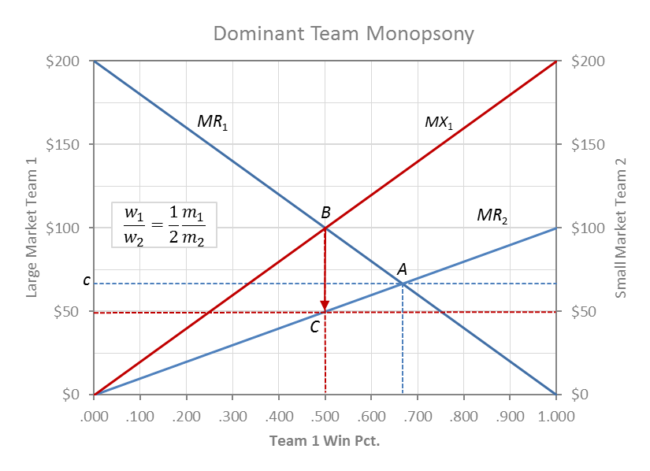
Monopsony Power Play
In the reality professional sports, the wage rate is probably not determined in a competitive labor market, but instead the going free agent rate is usually the rate that a dominant monopsony (one buyer) team sets at the beginning of the free-agency period.
In pursuit of monopsony maximum profit, team 1 can strategically lower the wage rate and cut payroll through the imposition of a salary cap that more than more than makes-up the difference in lost revenue from lower team quality and tanking.
In the process, team 2 will be allowed to acquire relatively more talent and win more games by also paying a lower non-competitive wage rate along MR2. A salary cap increases competitive balance within the league through a profit maximizing monopsony power play for both large and small market owners that comes at the negative-sum expense of players and large market fans.
The graph above shows the more likely case that a dominant monopsonist sets its wage rate just above the most that small market team 2 can pay along its demand curve MR2. In a monopsony labor market, MR2 demand curve for team 2 becomes the wage-setting labor supply curve for team 1 such that, c1 = MR2 = m2 w1.
Maximum profit requires MR1 = m1 w2 = 2m2 w1 = MX1 (marginal expenditure) at point B in the graph. The profit max competitive balance for a monopsonist is w1/w2 = m1/2m2, and if m1/m2 = 2 then w1/w2 = 1 and w1 = w2=.500.
Both teams pay the wage rate of c = 50 and carry equal payrolls 50 w1 = 50 w2 at point C. Both clubs are more profitable under monopsony, but it comes at the expense of the exploitation of players (the rectangle between c and 50 for both teams) and the lost welfare of fans (triangle ABC).
Visually, team 1 revenue declines by the area of the trapezoid under MR1 from A to B as team 1 dives into the tank. But team 2 winning only increases its revenue by the area of the trapezoid under MR2 from A to C because it is playing in a smaller market. The net welfare loss for fans overall is the triangular area ABC between MR1 and MR2.
Team 1 more than compensates its triangular loss in profit between MR1 and c above .500 with a net gain from rectangular payroll reduction between (c – 50) for w1 = .500. Team 2 is unambiguously more profitable with more revenue from winning and lower wage rate. Again the monopsony gains for both clubs come at the expense of the welfare of the players and large market fan base.
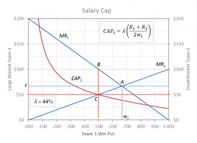
Winners and Losers
The graph above shows a salary cap set to constrain team 1 and impose absolute competitive balance .500/.500 at C on an competitively unbalanced league at A .667/.333. Under the competitive balance cap, team 1 cannot go above the rectangular hyperbola CAP1 = λ (C1 + C2)/ (2w1). The constrained salary cap solution is the point C where CAP1 = MR2.
(Team 2 also has a cap constraint CAP2 = λ (C1 + C2)/ (2w2), but it is not shown because team 2 is not constrained at A. See Two to Tango)
Anywhere along the hyperbolic CAP1 the payroll for team 1 is equal to the cap for the average team. The cap is a λ percentage of the average revenue team and so the actual cap payroll is actually a smaller percentage of large market team 1 revenue than small market team 2.
Under the cap, team 1 has lower revenue from winning fewer games but its profit margins are more than compensated by a reduction in player costs. Team 2 is more profitable both because it is winning more games and paying the players less. The players are paid less (c-50) and the lost welfare for team 1 fans is not compensated by the increased welfare for team 2 fans (ABC). (Fan preference for competitive balance is already revealed in the downward slope of the MR curves).
The profit maximizing cap percentage for Team 1 can be found by setting CAP1 = MR2. If m1/m2 = 2 then a players share of λ = 44.4% of revenue will maximize the profits of the monopsony league.
In this case the salary cap number is C = .250 for each team which is 44.4% of the league average revenue of TR / 2 = .5625. This cap number is actually 66.7% of the revenue of team 2 (R2 = .375) while being only 33.3% of the revenue of team1 (R1 = .750).
For example, the NFL Dallas Cowboys are the most valuable sports franchise in the world in 2019 at $5.5 billion, while paying its players $190 million – only 20 percent of its $950 million in revenue – and after having won an average .4 games over .500 (.525) since 2000. By comparison, the actual NFL players share of $220 million per average team in 2019 was capped at 48.6% of $452 million in average NFL revenue. (See comparison chart below).
In the final analysis, the tactical purpose of the salary cap is to protect large market teams in a collusive monopsony cartel against competition with themselves and maverick small market sportsmen (“cheating on the cartel”). Winners and losers from the monopsony salary cap power play are shown below for m1/m2 = 2 and here for other ratios of market size.
Monopoly league cartels on the demand (revenue) side are created by revenue sharing where the degree of cartelization is equal to the proportion of revenue that is shared among clubs. (NFL = 60%, MLB = 50%, NBA = 40% and NHL = 20%. See the GRID.) For the combined effects of the salary cap, revenue sharing and a payroll minimum see Two to Tango.
Optimum Salary Cap Effects for m1/m2 = 2 |
|||
| No Cap | λ = 44.4% | % Change | |
| m1/m2 | 2.00 | 2.00 | 0.0% |
| w1 | 0.667 | 0.500 | -25.0% |
| w2 | 0.333 | 0.500 | 50.0% |
| R1 | $0.889 | $0.750 | -15.6% |
| R2 | $0.278 | $0.375 | 35.0% |
| c | $0.667 | $0.500 | -25.0% |
| C1 | $0.444 | $0.250 | -43.8% |
| C2 | $0.222 | $0.250 | 12.5% |
| π1 | $0.444 | $0.500 | 12.5% |
| π2 | $0.056 | $0.125 | 125.0% |
| TR | $1.167 | $1.125 | -3.6% |
| TC | $0.667 | $0.500 | -25.0% |
| Tπ | $0.500 | $0.625 | 25.0% |
| John Vrooman /Vanderbilt | |||
Actual Player Shares
Actual player shares of revenues for 2018-19 are roughly similar to 44.4% in all Big 4 leagues:
Big 4 Player Expenses 2018-19 ($M) |
||||
| MLB | NFL | NBA | NHL | |
| League | ||||
| Total Revenue | $9,895 | $14,476 | $8,759 | $5,086 |
| Player Expense | $4,640 | $7,038 | $3,952 | $2,445 |
| % Players | 46.9% | 48.6% | 45.1% | 48.1% |
| Team | ||||
| Average Revenue | $329.8 | $452.4 | $292.0 | $164.1 |
| Player Expense | $154.7 | $219.9 | $131.7 | $78.9 |
| Salary Cap / Tax Threshold | $197.0 | $177.2 | $123.7 | $79.5 |
| Source: Forbes and John Vrooman /Vanderbilt.
NFL and NHL: slightly over 10% of player share goes to benefits before the cap is determined. NBA: 5 teams paid $156.7m luxury taxes in 2018-19. About 10% of players share goes to benefits before cap MLB: only 2 clubs paid $14.3m luxury taxes in 2018 down from five in 2017 and six in 2016. After paying the tax for 15 straight years, the New York Yankees and LA Dodgers (5 yrs) avoided it in 2018. Luxury tax:20% of payroll over $195M, $197M ,$206M, $208M, $210M (2017-21); 30%-50% for 2nd& 3rd breach; 12% surtax $20M – $40M; 42.5% over $40M. |
||||
Top to Bottom Value and Revenue Ratios
A market size ratio of m1/m2 = 2 yields a revenue ratio of R1/R2 = .750/.375 = 1.5 when the cap is set λ = 44.4% which is also consistent with the evidence.
Top 10 / Bottom 10 Value and Revenue Ratios ($M) |
||||
| MLB | NFL | NBA | NHL | |
| Team Value | ||||
| Top 10 | $2,713 | $3,700 | $3,168 | $1,057 |
| Bottom 10 | $1,119 | $2,153 | $1,451 | $454 |
| Ratio | 2.43 | 1.72 | 2.18 | 2.33 |
| Team Revenue | ||||
| Top 10 | $258 | $402 | $247 | $139 |
| Bottom 10 | $440 | $536 | $353 | $211 |
| Ratio | 1.71 | 1.33 | 1.43 | 1.52 |
| Source: Vrooman and Forbes. Revenue after sharing 2018-19. | ||||
Competitive Balance
Competitive balance can be interpreted and measured two ways: a Competitive Balance Index measures the distribution of wins within a given season and a Beta Balance Index which measures the continuity of wins and losses from season to season.
The CBI is the standard deviation in wins σ adjusted for season length (CBI = .5 / σ n^.5). Adjustment is necessary because according to law of large numbers, σ naturally decreases with more observations (games). The CBI ranges from 0 for a polarized league to 1 for a random league.
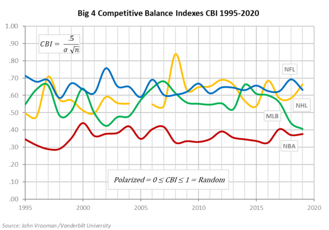
The chart above shows the CBI measures for the Big 4 leagues since the NFL Hard cap in 1995. The hard-cap constrained NFL is the most balanced league joined by the NHL after the inception of its hard cap in 2006. The soft-capped NBA is clearly the least balanced league joined recently by the uncapped MLB.
Beta Balance
Beta balance is an auto-regressive coefficient relating the win% between seasons: w t = β w t-1. β ranges from 0 for a fair chance every season to 1 for predetermined year to year dynasties and doormats.
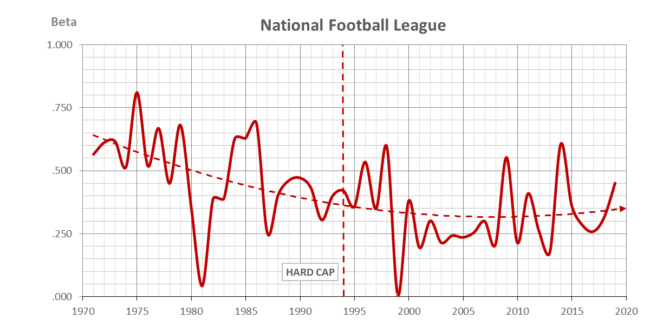
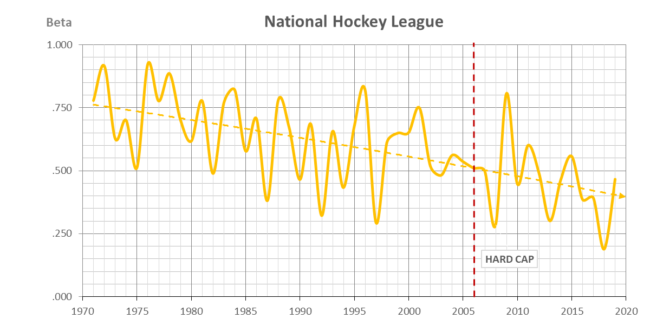
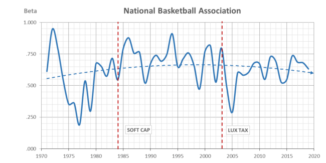
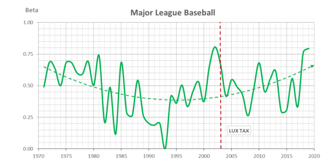
Beta balance auto-regressive coefficients (0 ≤ β ≤ 1) are shown above since the AFL-NFL merger in 1970 with similar results to the CBI. The hard-capped NFL and NHL are the most balanced from season to season (β < .5) and it can be traced to the inception of the hard cap for the NFL in 1994 and the NHL in 2006. The NBA is clearly the most predetermined and it has been joined in the last two seasons by MLB (β > .5).
Big 4 Salary Cap / Luxury Tax Histories: Big 4 Cap History / Cap Graphs / Combo
NBA Salary Cap & Luxury Tax |
|||
| Year | Salary Cap | Minimum | Luxury Tax |
| 2020-21 | $115.0 | $103.5 | $139.0 |
| 2019-20 | $109.1 | $98.2 | $132.6 |
| 2018-19 | $101.9 | $91.7 | $123.7 |
| 2017-18 | $99.1 | $89.2 | $119.3 |
| 2016-17 | $94.1 | $84.7 | $113.3 |
| 2015-16 | $70.0 | $63.0 | $84.7 |
| 2014-15 | $63.1 | $56.8 | $76.8 |
| 2013-14 | $58.7 | $52.8 | $71.7 |
| 2012-13 | $58.0 | $52.2 | $70.3 |
| 2011-12 | $58.0 | $52.2 | $70.3 |
| 2010-11 | $58.0 | $52.2 | $70.3 |
| 2009-10 | $57.7 | $51.9 | $69.9 |
| 2008-09 | $58.7 | $52.8 | $71.2 |
| 2007-08 | $55.6 | $50.1 | $67.9 |
| 2006-07 | $53.1 | $47.8 | $65.4 |
| 2005-06 | $49.5 | $44.6 | $61.7 |
| 2004-05 | $43.9 | $39.5 | … |
| 2003-04 | $43.8 | $39.5 | $54.6 |
| 2002-03 | $40.3 | $36.2 | $52.9 |
| 2001-02 | $42.5 | $38.3 | … |
| 2000-01 | $35.5 | $32.0 | … |
| 1999-00 | $34.0 | $30.6 | … |
| 1998-99 | $30.0 | $27.0 | … |
| 1997-98 | $26.9 | $24.2 | … |
| 1996-97 | $24.4 | $21.9 | … |
| 1995-96 | $23.0 | $20.7 | … |
| 1994-95 | $16.0 | $14.4 | … |
| 1993-94 | $15.2 | $13.7 | … |
| 1992-93 | $14.0 | $12.6 | … |
| 1991-92 | $12.5 | $11.3 | … |
| 1990-91 | $11.9 | $10.7 | … |
| 1989-90 | $9.8 | $8.8 | … |
| 1988-89 | $7.2 | $6.5 | … |
| 1987-88 | $6.2 | $5.5 | … |
| 1986-87 | $4.9 | $4.5 | … |
| 1985-86 | $4.2 | $3.8 | … |
| 1984-85 | $3.6 | $3.2 | … |
| NBA: Soft cap since 1984-85: 49-51% of BRI. Minimum 90% of cap. Cap set at 44.74% of expected BRI. Luxury tax threshold set at 53.5% BRI. | |||
NFL Salary Cap |
||
| Year | Salary Cap | Minimum |
| 2021 | ||
| 2020 | $198.2 | $178.4 |
| 2019 | $188.2 | $169.4 |
| 2018 | $177.2 | $159.5 |
| 2017 | $167.0 | $150.3 |
| 2016 | $155.3 | $139.7 |
| 2015 | $143.3 | $129.0 |
| 2014 | $133.0 | $119.7 |
| 2013 | $123.0 | $110.7 |
| 2012 | $120.6 | $108.5 |
| 2011 | $120.0 | $108.0 |
| 2010 | Uncapped | |
| 2009 | $123.0 | $110.7 |
| 2008 | $116.0 | $104.4 |
| 2007 | $109.0 | $98.1 |
| 2006 | $102.0 | $91.8 |
| 2005 | $85.5 | $77.0 |
| 2004 | $80.6 | $72.5 |
| 2003 | $75.0 | $67.5 |
| 2002 | $71.1 | $64.0 |
| 2001 | $67.4 | $60.7 |
| 2000 | $62.2 | $56.0 |
| 1999 | $57.3 | $51.6 |
| 1998 | $52.4 | $47.1 |
| 1997 | $41.5 | $37.3 |
| 1996 | $40.8 | $36.7 |
| 1995 | $37.1 | $33.4 |
| 1994 | $34.6 | $31.1 |
| NFL Hard cap since free agency in 1994 CBA: 48-48.8% of all revenue Cap includes prorated bonuses. Minimum payroll 89% of cap. | ||
NHL Salary Cap |
|||
| Season | Salary Cap | Minimum | Mid-point |
| 2020-21 | |||
| 2019-20 | $81.5 | $60.2 | $70.9 |
| 2018-19 | $79.5 | $58.8 | $69.1 |
| 2017-18 | $75.0 | $55.4 | $65.2 |
| 2016-17 | $73.0 | $54.0 | $63.5 |
| 2015-16 | $71.4 | $52.8 | $62.1 |
| 2014-15 | $69.0 | $51.0 | $60.0 |
| 2013-14 | $64.3 | $47.5 | $55.9 |
| 2012-13 | $60.0 | $44.3 | $52.2 |
| 2011-12 | $64.3 | $47.5 | $55.9 |
| 2010-11 | $59.4 | $43.9 | $51.7 |
| 2009-10 | $56.8 | $42.0 | $49.4 |
| 2008-09 | $56.7 | $41.9 | $49.3 |
| 2007-08 | $50.3 | $37.2 | $43.7 |
| 2006-07 | $44.0 | $32.5 | $38.3 |
| 2005-06 | $39.0 | $28.8 | $33.9 |
| NHL Hard cap since 2004-05 lockout: 50% of hockey related revenue HRR. Cap and min are +/- 15% of midpoint | |||
MLB Luxury Tax |
|
| Year | Luxury Tax |
| 2021 | $210.0 |
| 2020 | $208.0 |
| 2019 | $206.0 |
| 2018 | $197.0 |
| 2017 | $195.0 |
| 2016 | $189.0 |
| 2015 | $189.0 |
| 2014 | $189.0 |
| 2013 | $178.0 |
| 2012 | $178.0 |
| 2011 | $178.0 |
| 2010 | $170.0 |
| 2009 | $162.0 |
| 2008 | $155.0 |
| 2007 | $148.0 |
| 2006 | $136.5 |
| 2005 | $128.0 |
| 2004 | $120.5 |
| 2003 | $117.0 |
| Lux Tax: Under 2002 and 2006 agreements, first time violators were charged a 17.5% to 22.5% tax, second-time offenders a 30% tax, and three-time a 40% tax. additional penalty was added in 2012 CBA, taxing teams that exceed the threshold for four or more years in a row at a 50% rate. | ||||||
| MLB CBA: 2017-21. Tax rates are 20 percent for first-time payors, 30 percent for second-time payors, and 50 percent for payors exceeding the threshold for a third consecutive season or more. In addition, MLB will levy a surtax on clubs exceeding the threshold by $20 million or $40 million. |
©2025 Vanderbilt University · John Vrooman
Site Development: University Web Communications