Software: Download DSI Studio
Instructions:
(If you already have a subject .fib file in Talairach space such as that produced during preprocessing, proceed to Step #3.)
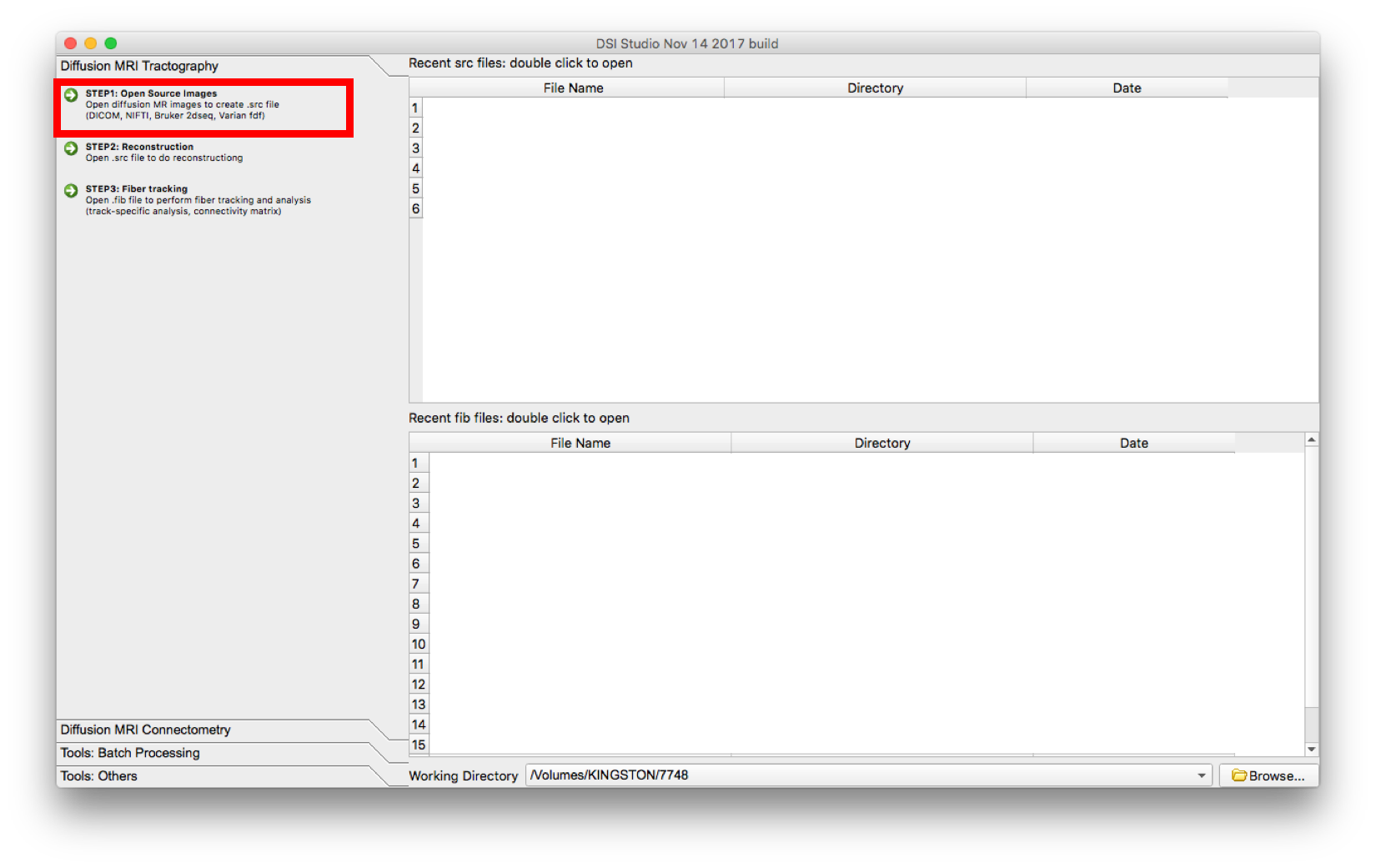
- Select “Step 1: Open Source Image” to load diffusion MR images (DICOM, NIFTI, Bruker 2dseq, Varian fdf) in order to create a .src file. The .src will be created and located in the main window
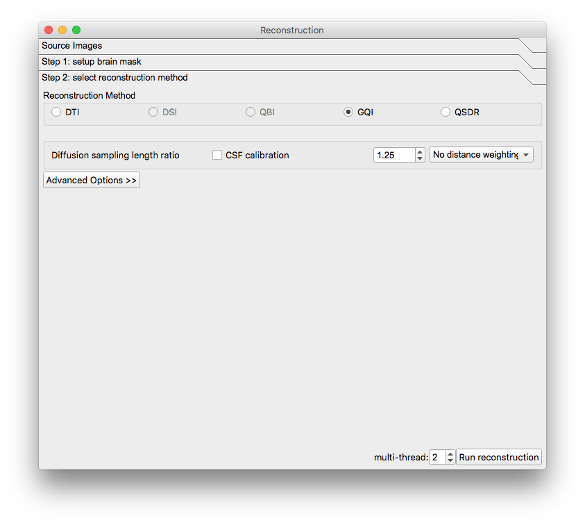
- Select “Step 2: Reconstruction”
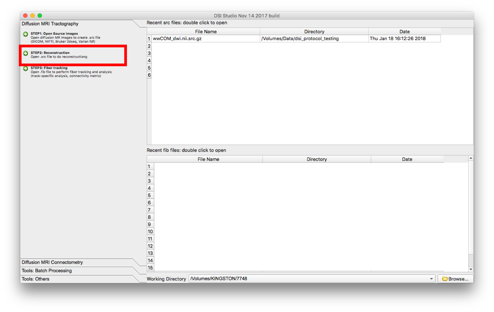 A new window will appear. Confirm the appearance of the mask and select the reconstruction method to be GQI. The reconstructed image will appear in the main window but it will have a filename ending in “.src.gz”.
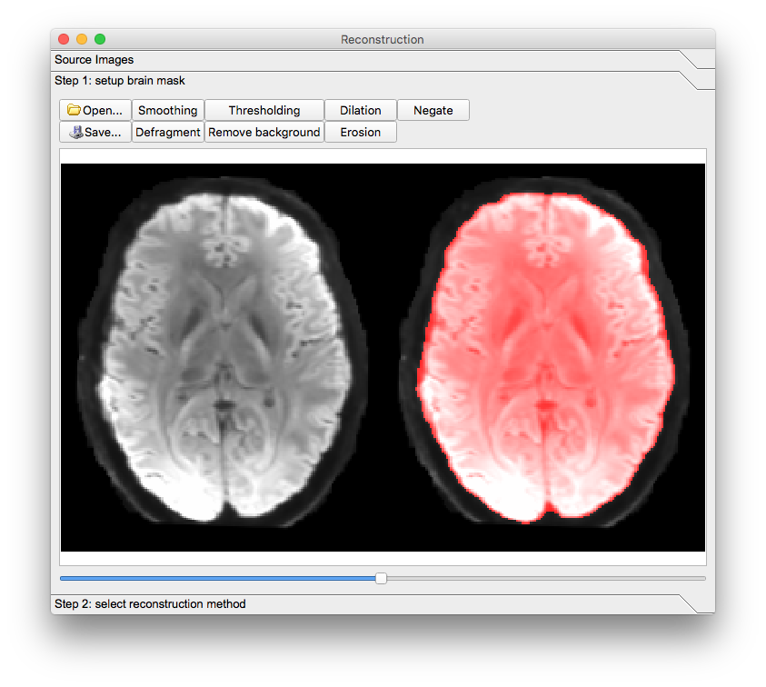
- Select “Step 3: Fiber Tracking” and open the subject .fib file.
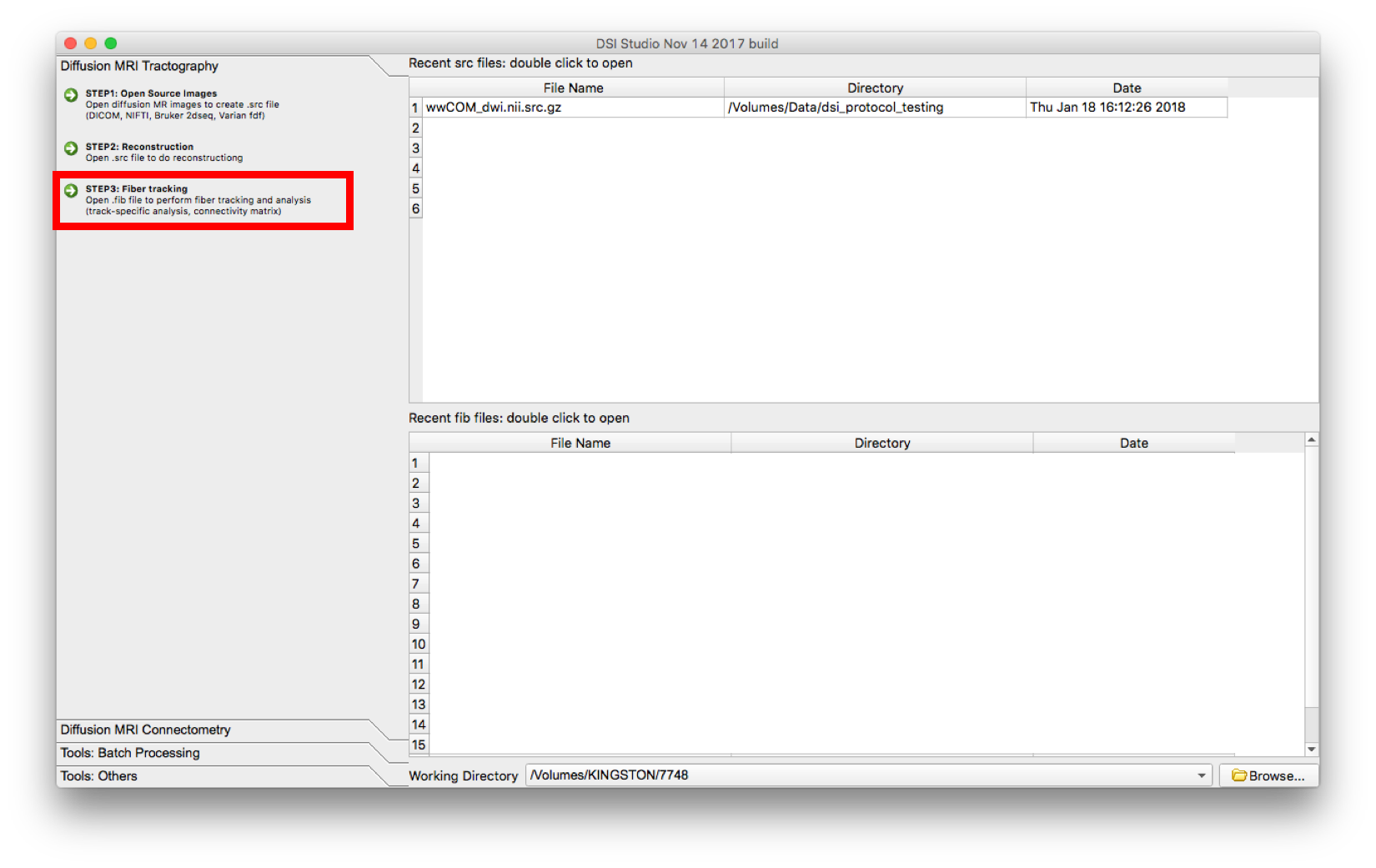
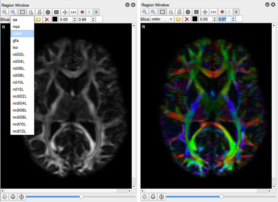
The following screens will appear: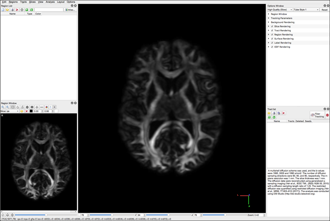
- Select “color” under the Slice dropdown menu
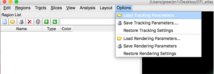
- Load this Tracking Parameters file into dsi studio.
 The tracking parameters settings should be:
- Termination Index = nqa
- Threshold = 0.1
- Angular Threshold = 0
- Step Size(mm) = 0.0
- Smoothing = 1.0
- Min length(mm) = 30.0
- Max length(mm) = 300.0
- Seed Orientation = primary
- Seed Position = subvoxel
- Randomize Seeding = off
- Check Ending = off
- Direction Interpoation = trilinear
- Tracking Algorithm = stremline(euler)
- Terminate if = 100,000 tracts
- Thread Count = 2
- Output Format = trk.gz
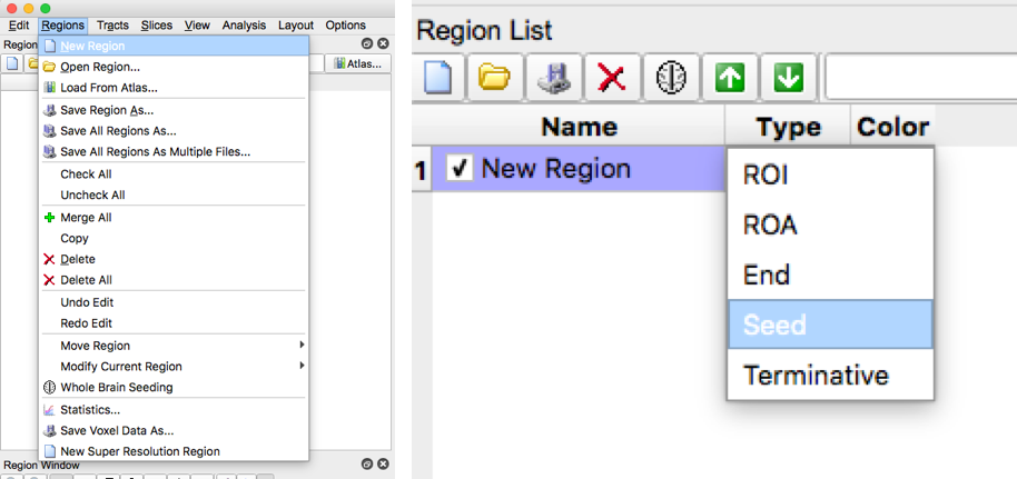
- For each brain slice create a new region. In generally, you should have about 1-2 seed regions per tract and 0-2 roi regions per tract. Under type, select “seed” for seed regions, or select “ROI” for roi regions
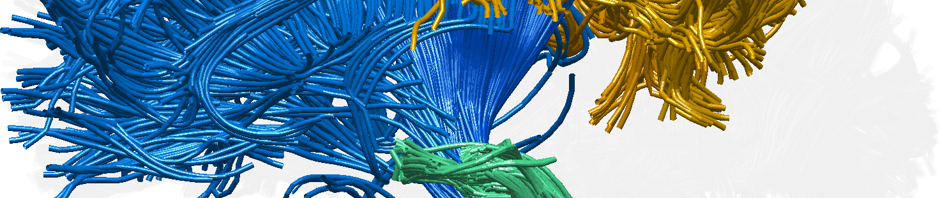
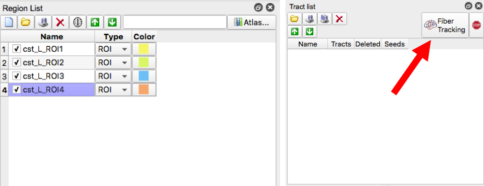
- Please review the diagram below to acquaint yourself with the software
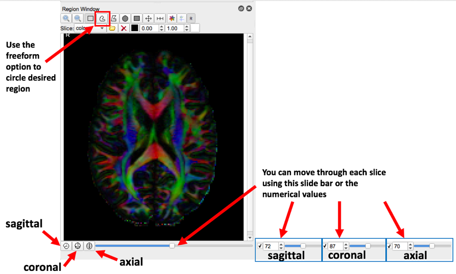
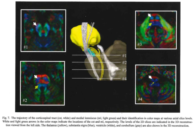
- Our first example tract is the corticospinal tract, referenced in Fig.7 of MRI Atlas of Human White Matter 2nd Ed. To begin, move the axial slide bar until you reach a slice that looks similar to one of the boxes. Then using the freeform option, make a circle around the region that the arrow is pointing to. Follow these two steps for the remaining three boxes. Be sure to make a new region with each slice (in this case, for each box)
- Make sure all four ROI regions are checked then select “Fiber Tracking”
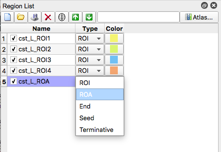
- If the resulting tract does not look like the picture in Figure 7. Create exclusion regions to remove erroneous streamline fiber tracts. This achieved by creating a region and selecting “ROA”. Then, using the square or freeform option, enclose the region where the erroneous fiber is located (if applicable, you can place use the square option and cover the entire brain slice to exclude any fivers that go through that slice)
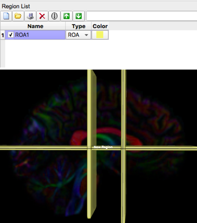
- For simplified bookkeeping purposes, all exclusion regions should be created using the same ROA region. For example, in the image below, three exclusion regions (two on a coronal slice, one on an axial slice) were drawn but only one ROA region was created.
- Final step, save all of the files: tract image, regions, and density image. Be sure to save it in the appropriate tract folder (e.g. corticiospinal_tract) and make sure the file names are unique. Renaming each file uniquely, following the naming system below
- ROIs: [tract abbreviation]_[L or R]_ROI{1,2,3,…} Example ROI on the right side: cst_R_ROI1, cst_R_ROI2, …
- Seeds: [tract abbreviation]_[L or R]_seed{1,2,3,…} Example seed on the right side: cst_R_seed1, cst_R_seed2, …
- ROAs: [tract abbreviation]_ROA{1,2,3,…} Example ROA on the right side: cst_R_ROA1
- Tracts: [tract abbreviation]_[L or R]_tract Example tract: cst_L_tract
- Density: [tract abbreviation]_[L or R]_density Example density: cst_L_density
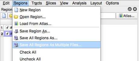
- Save the regions by selection “Save all regions as Multiple Files”, then select open when the appropriate folder location is created
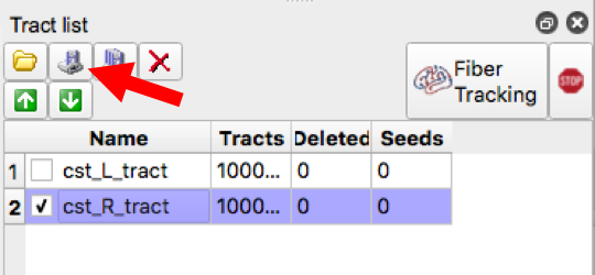
- Save the Tract Image (make sure only a single tract is checked in the tract list) then select the save button
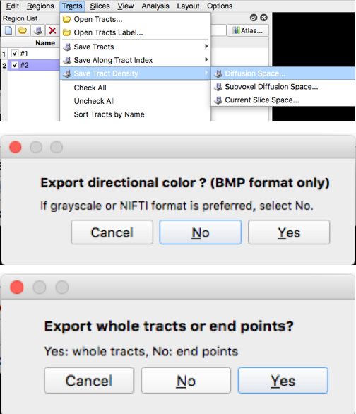
- Save the density map by selecting “tract Density Image” then “Diffusion Space”, Select “No” in response to whether to export directional color, then select “Yes” in response to exporting the whole tract (make sure only one tract is checked in the tract list each time you save the density image)